In search of a color

^[1]

Last week I found an intriguing book in the local charity shop (these are called ‘thrift shops’ in the US I think) for £1.00: Mauve, by Simon Garfield ^[2]. It’s a book all about the colour mauve, its discovery by William Perkin in the mid 19th century, and the story of the later scientific developments in industrial chemistry.

(By the way, the pronunciation of “mauve” may vary depending on where and when you live. Here in England we’d start by saying “mo” to rhyme with “go” and then finish by saying “-ve” as if we’d finished saying “love”. The Victorians pronounced it as if it was spelt “morv”.)

White, black, or one of the primary colours might be able to fill a book, but it’s unusual to find a whole book about a single shade of a colour. Although, there’s a bit of biography and plentiful helpings of the history of chemistry too.

It’s a great story (you might know it already). In London, in the 1850s, 18 year old chemistry student William Perkin has been assigned the task of synthesizing quinine from coal tar residues, as part of the effort to combat the ongoing worldwide malaria epidemic. Each attempt failed, but just before throwing out one particularly bad mess, he spotted a purple glint deep in the slurry. Seeing the potential, and against the advice of his supervisors, he left academia, set up a factory, obtained a patent (you could patent colors then), and by the end of the 1850s he was making a lot of money providing the new color to the clothing and dyeing industries.

As with many modern entrepreneurs, such as Steve Jobs or Bill Gates, there was a bit of luck too. It helped that he was in exactly the right place at exactly the right time. Because, shortly after he’d got his new start-up into production, there was a sudden European-wide craze for the color mauve. Queen Victoria wore it to a royal wedding, the Empress Eugenie, Napoleon III’s wife, made it fashionable in Paris. And these celebrity endorsements, then as now, drove sales to new heights. “Mauve mania” swept through Europe.

Let’s see what this amazing mauve color looks like on our modern machines. I loaded up the Julia colors package, Colors.jl, and set up a quick test:

using Colors, Luxor
@draw begin
    setcolor("mauve")
    paint()
end 600 300

ERROR: LoadError: Unknown color: mauve
Stacktrace:
 [1] error(::String, ::String) at ./error.jl:42
 [2] _parse_colorant(::String) at /Users/me/.julia/packages/Colors/r1p4Q/src/parse.jl:103
 [3] _parse_colorant(::Type{RGBA}, ::Type{ColorAlpha{RGB{T},T,4} where T<:Union{AbstractFloat, FixedPointNumbers.FixedPoint}}, ::String) at /Users/me/.julia/packages/Colors/r1p4Q/src/parse.jl:112
 [4] parse at /Users/me/.julia/packages/Colors/r1p4Q/src/parse.jl:145 [inlined]
 [5] setcolor(::String) at /Users/me/.julia/dev/Luxor/src/colors_styles.jl:29
 [6] top-level scope at untitled-ba17b354ac0d06ec10bd7374a7ef9522:4
 [7] top-level scope at /Users/me/.julia/dev/Luxor/src/drawings.jl:555
in expression starting at untitled-ba17b354ac0d06ec10bd7374a7ef9522:3

Oh, that didn’t go well. No sign of mauve? Mauve, one of the most famous colors of the 19th Century, has been put in the shade by colors with names like Burleywood and Papaya Whip.

Standards, what standards?

In Colors.jl, the list of named colors is essentially the X11/CSS standard list. Typing color names is definitely not the best way of specifying colors - obviously, values in the RGB, Luv, and HSV color spaces are more precise, as are those three or six figure hexadecimal codes. But it’s sometimes easier to quickly grab a color name - “gold”, say - than to start filling your head with hex or computer-y numbers. There’s a slight speed penalty for using the names, too (unless you use the macros), because they have to be parsed, but that won’t be a problem for many applications.

So what exactly qualifies a color for inclusion in the ‘official’ X11/CSS list? I was expecting to read about rigorous committee-driven meetings where each color was carefully scrutinized before being accepted as a standard, but in fact the X11 color list is famously imperfect and inconsistent, assembled in a haphazard way by assorted MIT hackers over the last few decades, with all kinds of quirks, oddities, and even errors. You can read an entertaining story of these color names here. Quoted there is one Steven Pemberton: ^[3]

“The X11 colour names are an abomination that should have been stifled at birth, and adding them to CSS is a blemish on the otherwise excellent design of CSS. To say that the X11 colour set and their names have been ‘designed’ is an insult to the word ‘design.’ It is just a mess.”

And later on:

Another point of contention was cultural exclusion. Some programmers took umbrage at the region-centric nature of names like “dodger blue” and the potential racial undertones of “navajo white” (from Sinclair Paints) and “indian red” (from Crayola, though the crayon has since been renamed in response to the same concerns). Others considered the English-only names alienating.

So it was just bad luck that mauve wasn’t part of a set of crayons and so didn't make it on to the list of standard colors.

Where is mauve?

I wanted to plot the X11 named colors all at once, to see where mauve might fit in. Using HSB color values, I tried making a polar plot: the hue angle places a marker somewhere on a disk, and the saturation can be the distance from the centre (0) to the circumference (1). The third value, brightness, can be drawn on an axis pointing straight out of the screen by using circles with decreasing radius as it approaches 1.

using Luxor, Colors
function circularlegend(pos, radius)
    @layer begin
        fontsize(10)
        sethue("gray50")
        circle(pos, radius, :stroke)
        for θ in range(0, 2π - π/12, step=π/12)
            label(string(convert(Int, round(rad2deg(θ), digits=1)), "°"), θ, polar(radius + 5, θ))
        end
        sethue("gray20")
        setline(.5)
        for (n, theta) in enumerate(range(0, 2π, step=π/12))
            line(polar(20, theta), polar(radius, theta), :stroke)
        end
    end
end

@svg begin
    background("black")
    rad = boxwidth(BoundingBox() * 0.9)/2
    circularlegend(O, rad)
    fontsize(2)
    dotstack = Tuple{Point, Colorant, Float64}[]
    for (k, v) in Colors.color_names
        r, g, b = 1/256 .* v
        col = convert(HSB, RGB(r, g, b))
        h, s, br = col.h, col.s, col.v
        radius = rescale(s, 0, 1, 0, rad)
        pt = polar(radius, 2π * h/360)
        push!(dotstack, (pt, col, br))
    end
    sort!(dotstack, by = x -> last(x))
    for dot in dotstack
        sethue(dot[2])
        circle(dot[1], rescale(dot[3], 0, 1, 10, 1), :fillstroke)
    end
end 800 800  "_assets/images/mauve/colornames.svg"

All the grey shades are stacked up at the center. The ‘spheres’ are created because a number of colors are basically the same hue and saturation but just differ in brightness, the out-of-the-screen dimension.

I think there’s a definite bias towards reds and oranges.

Rainbow warrior

We don't have to restrict ourselves merely to the X11/CSS list though. The Julia wizard known as oxinabox has compiled a much bigger collection of named colors, over at NamedColors.jl.

using NamedColors

@svg begin
   background("black")
   rad = boxwidth(BoundingBox() * 0.9)/2
   circularlegend(O, rad)
   dotstack = Tuple{Point, Colorant, Float64, String}[]
   for (k, v) in NamedColors.ALL_COLORS
       col = convert(HSB, v)
       h, s, br = col.h, col.s, col.v
       radius = rescale(s, 0, 1, 0, rad)
       pt = polar(radius, 2π * h/360)
       push!(dotstack, (pt, col, br, k))
   end
   fontsize(8)
   sort!(dotstack, by = x -> x[3])
   setline(2)
   for dot in dotstack
        pt, col, br, k = dot
        d = rescale(br, 0, 1, 8, 1)
        sethue(col)
        circle(pt, d/2, :fillstroke)
   end
end 800 800  "_assets/images/mauve/namedcolornames.svg"

Some of these do have mauve in the names, so we can isolate them by replacing two lines with:

if occursin("mauv", k)
    sethue("cyan")
    box(pt, 2d, 2d, :stroke)
    text(k, pt + (0, 8), halign=:center)
    sethue(col)
    circle(pt, d/2, :fillstroke)
end

If you ask me, I don’t think many of these are really mauve. There’s a sparse-looking area in the purples where I think a real mauve might belong. So, what color is mauve? To find out, I think we’ll have to go back in time.

The royal purple

When Perkin first thought of naming his new discovery, he settled for Tyrian Purple. This is the famous rich purple color much prized by the Romans, which could only be worn by nobles and emperors. It was fabulously expensive to make (only tiny amounts could be extracted from the glands of hundreds of thousands of a particular species of mollusc), was sometimes more expensive than gold, and was occasionally compared to the color of dried blood. Presumably Perkin’s new colour was similar enough to a rich purple to justify his choice of name? Or was he just trying to boost the commercial prospects of his pale pseudo-royal purple dye?

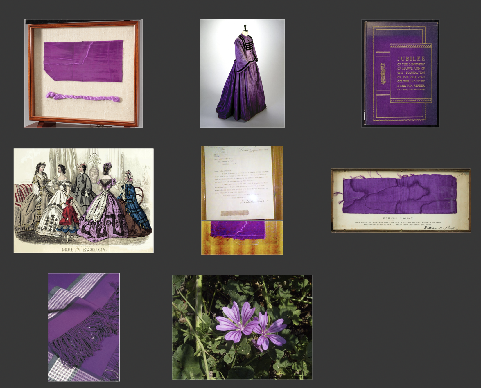
Let’s get some visual help, and see about getting some values. I’m unable to do any real scientific analysis with expensive machines and things ^[4], so I just found a few relevant images featuring mauve, and played around with the pixel values, looking for clues. The pictures at top left, center, and middle right show original samples of fabric dyed with mauveine, the mauve dye. At bottom left is a scarf or shawl. For good measure I found pictures of a couple of dresses, one real and one in a painting, and a book. At the bottom is the Mallow flower; the word mauve is the French name of this flower.

^[5]

Then I hacked up a bit of code to process the images and look for the colors. It’s a bit prototype-y at the moment.

using Images

function project(x, y, z;
        sf = 3, hm = -1)
    # negative because y is positive downwards
    u = (x - y)/sqrt(2)
    v = (x + 2(hm * z) + y)/sqrt(6)
    return Point(sf * u, sf * v)
end
project(t; kwargs...) = project(t[1], t[2], t[3]; kwargs...)

function drawisoaxes(;
        sf = sf,
        hm = hm, r = 300)
    @layer begin
        fontsize(14)
        setline(0.5)
        p = project(0, r, 0, sf = sf, hm = hm)
        line(project(0, -r, 0, sf = sf, hm = hm), p, :stroke)
        text("y", p)
        p = project(r, 0, 0, sf = sf, hm = hm)
        line(project(-r, 0, 0, sf = sf, hm = hm), p, :stroke)
        text("x", p)
        p = project(0, 0, r, sf = sf, hm = hm)
        line(project(0, 0, -r, sf = sf, hm = hm), p, :stroke)
        text("z", p)
    end
end

function drawimagefile(imfile;
        caption="caption")
    background("grey10")
    img = load(imfile)
    panels = Table([700], [550, 400])
    subpanels = Table([450, 250], [390], panels[2])
    sf = 0.8
    hm = -1
    S = panels.colwidths[1]/2 - 50
    S1 = subpanels.colwidths[1] - 10
    # at left, a top down view
    @layer begin
        translate(panels[1])
        circularlegend(O, S)
    end
    # store not draw
    dotstack = Tuple{Point, Colorant, Float64}[]
    isostack = Tuple{Point, Colorant, Float64}[]
    for i in img
        r, g, b = i.r, i.g, i.b
        col = convert(HSB, RGB(r, g, b))
        h, s, v = col.h, col.s, col.v
        radius = rescale(s, 0, 1, 0, S)
        height = rescale(v, 0, 1, 0, S)
        pt = polar(radius, 2π * h/360)
        ptiso = project(pt.x, pt.y, height, sf = sf, hm = hm)
        depth = pt.x + pt.y + height
        push!(isostack, (ptiso, col, depth))
        push!(dotstack, (pt, col, height))
    end
    @layer begin
        translate(subpanels[1])
        sethue("gray90")
        drawisoaxes(sf = sf, hm = hm, r = S1/2)
    end
    # sort and draw
    @layer begin
        sort!(dotstack, by = x -> last(x))
        translate(panels[1])
        for d in dotstack
            setcolor(d[2])
            circle(d[1], 1, :fill)
        end
    end
    @layer begin
        sort!(isostack, by = x -> last(x))
        translate(subpanels[1])
        for d in isostack
            setcolor(d[2])
            circle(d[1], .5, :fill)
        end
    end
    # thumbnail
    @layer begin
        translate(subpanels[2])
        # need PNGs for Luxor, cos Cairo don't do JPG :(
        save("/tmp/img.png", img)
        img = readpng("/tmp/img.png")
        panelsize = min(subpanels.rowheights[2], subpanels.colwidths[1])
        @layer begin
            scale(1 / (1.1 * max(img.width, img.height) / panelsize))
            placeimage(img, O, centered=true)
        end
    end
    # title
    @layer begin
        sethue("white")
        fontsize(24)
        fontface("AvenirNext-Bold")
        text(caption, boxtopcenter(BoundingBox(box(panels, 1))) + (0, 25),
            halign=:center)
    end
end

And it runs like this:

@png begin
        background("grey10")
        drawimagefile("_assets/images/mauve/science-museum-f6.jpg", caption="fabric")
end 1200 900 "_assets/images/mauve/fabricsample.png"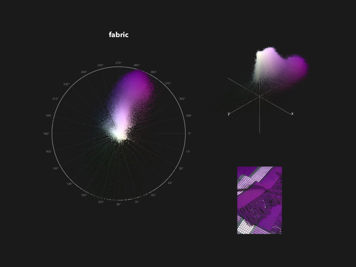

In this image, each pixel of the original is drawn three times - in the thumbnail, on an isometric projection of the Hue/Saturation/Brightness space, and again on the Hue wheel as before.

Here are the other images:

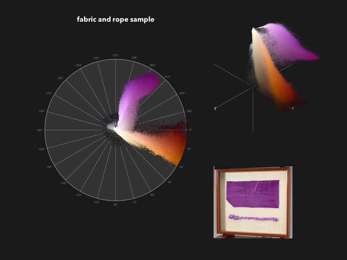
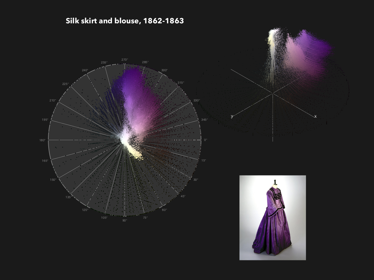
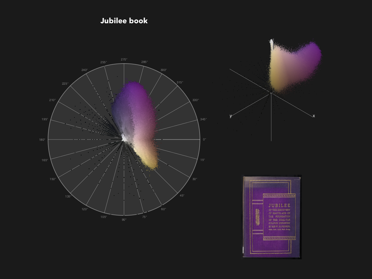
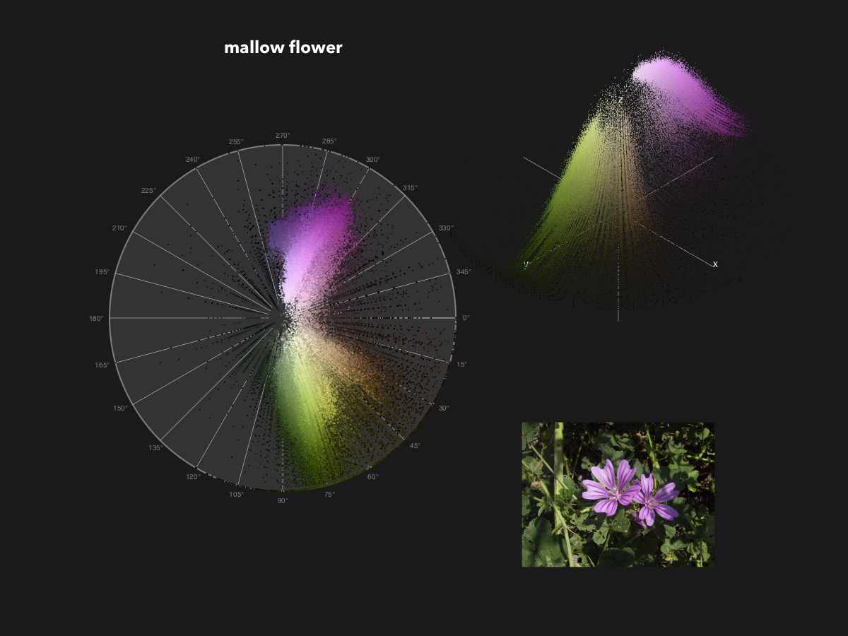
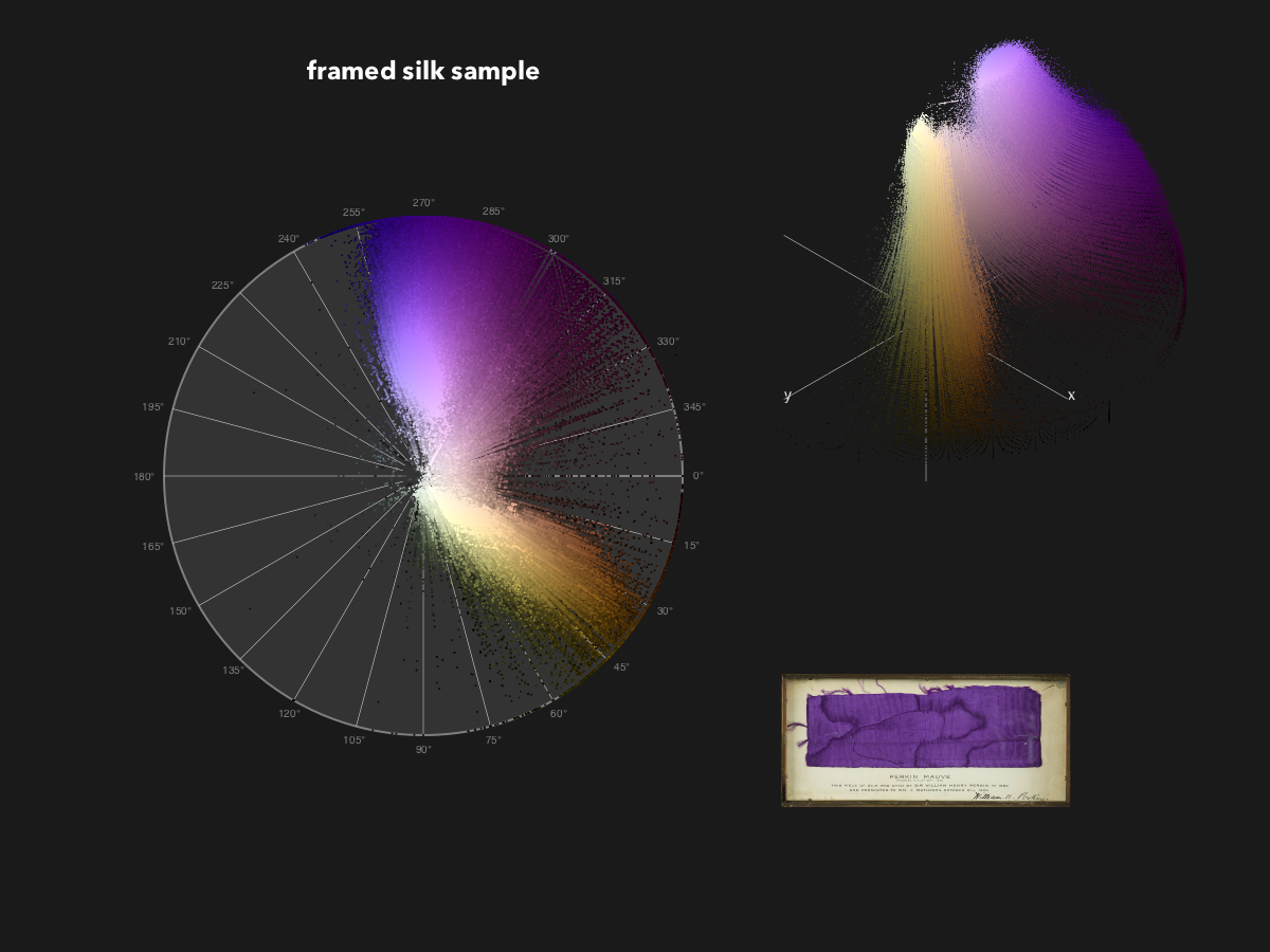
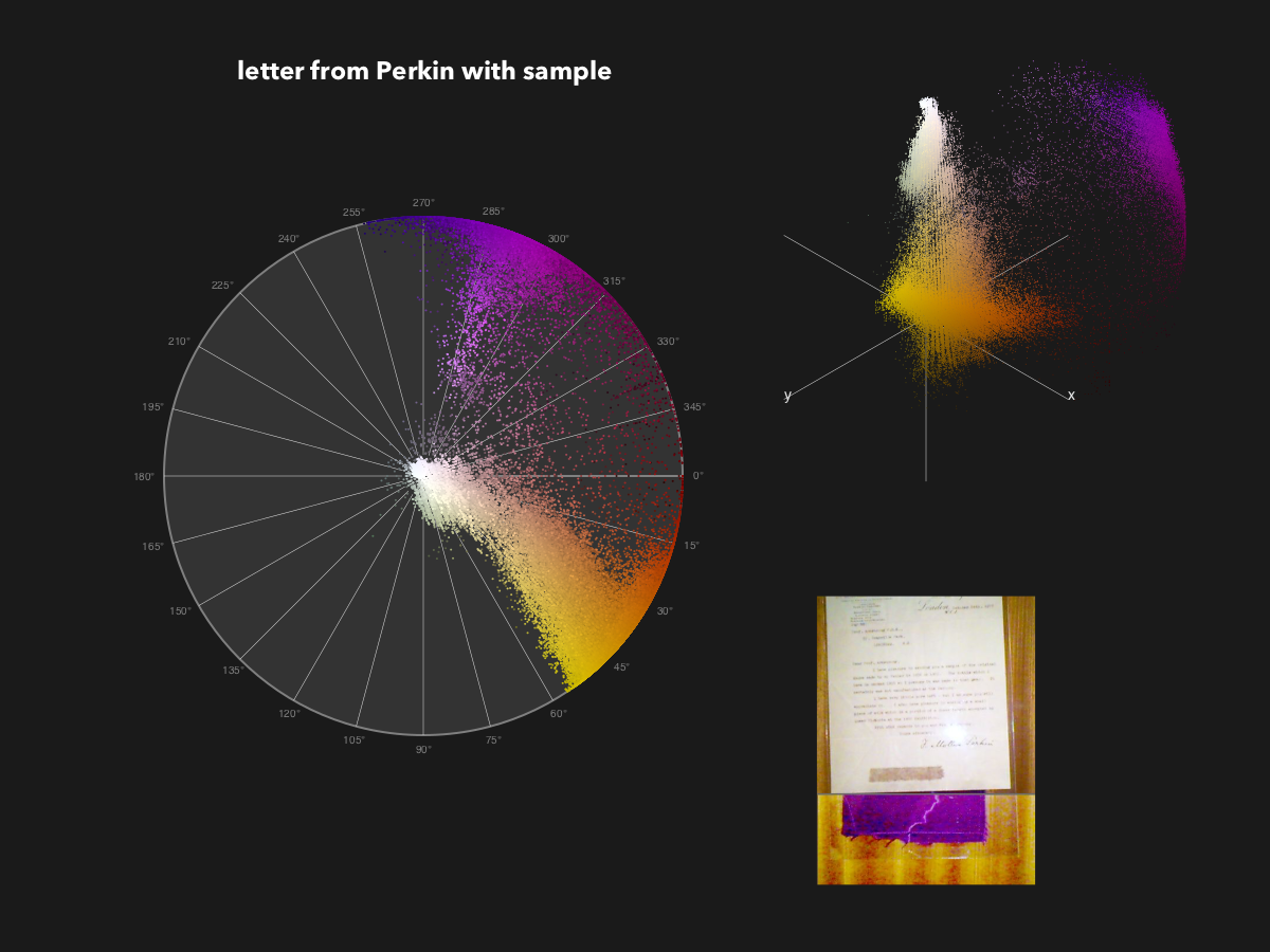
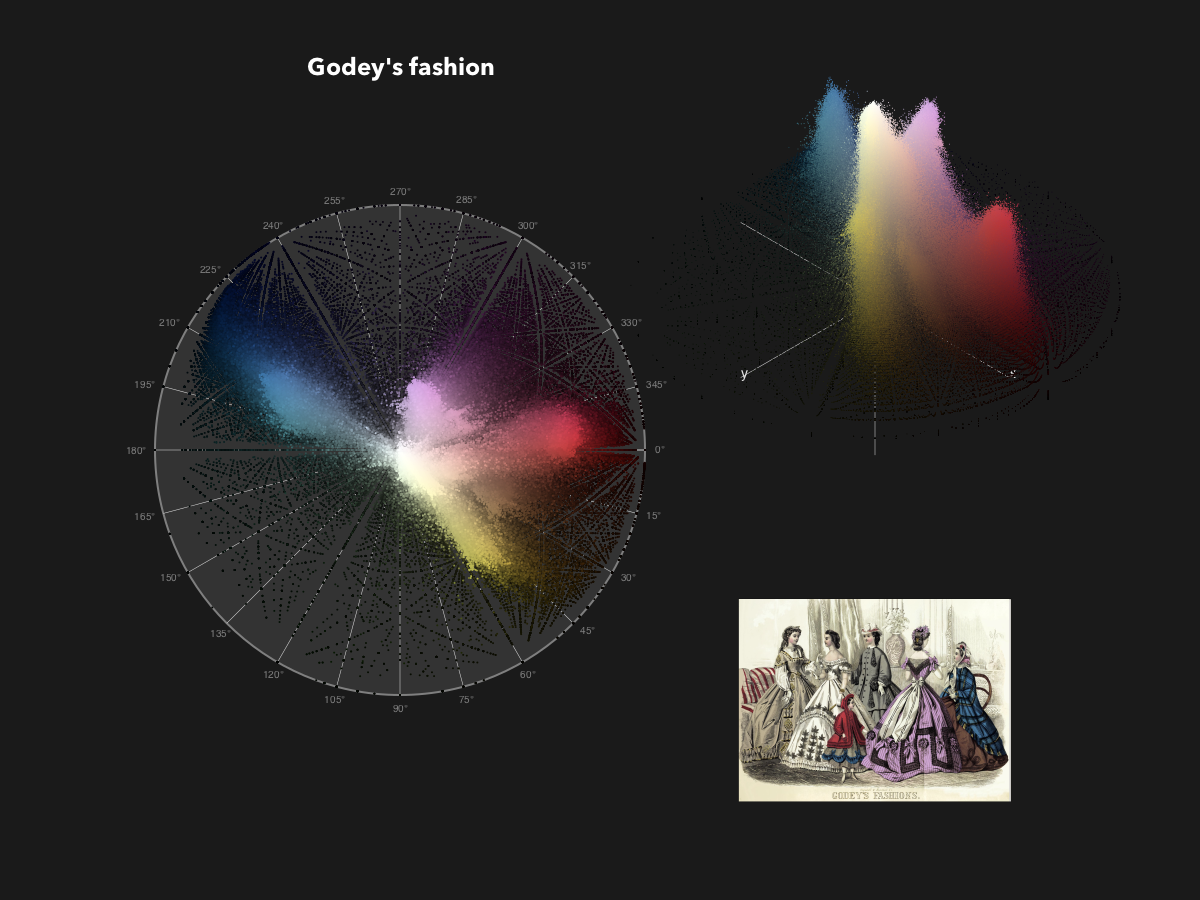
So my initial guess from eye-balling these is that mauve should be about HSB(277.5, 0.75, 0.85) - give or take a bit. (I’d like to do some statistics to confirm or challenge this but perhaps that’s for a follow-up post...)

@svg begin
    background("black")
    rad = boxwidth(BoundingBox() * 0.9)/2
    circularlegend(O, rad)
    for sat in 0.9:-0.025:0.5
        for r in 270:2:285 ## degrees
            brightness = .85
            sethue(HSB(r, sat, brightness))
            mauvepos = polar(rescale(sat, 0, 1, 0, rad), deg2rad(r))
            circle(mauvepos, 3, :fill)
        end
    end
end 800 800 "_assets/images/mauve/mauvepoints"

Somewhere around here perhaps?

50 shades of ... mauve

To find the nearest named color to what I think the original mauve would have been, I used the colordiff() function from Colors.jl. It’s probably a reasonable approximation to the truth.

function findnearestcolors(sourcecol::Colorant, matches=3, colordict=Colors.color_names)
    results = Float64[]
    names = String[]
    for (k, v) in colordict
        if typeof(v) == Tuple{Int64,Int64,Int64}
            r, g, b = v ./ 256
            tempcol = convert(HSB, RGB(r, g, b))
        elseif typeof(v) == RGB24
            tempcol = convert(HSB, v)
        end
        push!(results, colordiff(sourcecol, tempcol))
        push!(names, k)
    end
    return results[sortperm(results)[1:matches]], names[sortperm(results)[1:matches]]
end

Here’s the code to make a table of them:

function drawclosestcolors(targetcolor, numberofcolors = 30, colordict = Colors.color_names;
        title = "color")
    distances, colornames = findnearestcolors(targetcol, numberofcolors, colordict)
    t = Tiler(600, 600, numberofcolors, 1, margin=60)
    for (pos, n) in t
        # draw target color in left column
        sethue(targetcol)
        box(pos - (t.tilewidth/4, 0), t.tilewidth/4, t.tileheight - 2, :fill)
        # draw near color in right column
        dist = rescale(distances[n], extrema(distances)..., 1, 30)
        if typeof(colordict[colornames[n]]) == Tuple{Int64, Int64, Int64}
            matched = colornames[n]
        else
            matched = colordict[colornames[n]]
        end
        sethue(matched)
        box(pos + (dist + t.tilewidth/4, 0), t.tilewidth/2, t.tileheight - 2, :fill)
        # add some text too
        sethue("white")
        mh, ms, mv = round.(getfield.(convert(HSV, parse(Colorant, matched)), 1:3), digits=2)
        text(string(
                colornames[n],
                " ($mh $ms $mv) ",
                round(distances[n], digits=2)),
            pos + (t.tilewidth/2, 0), halign=:right, valign=:middle)
    end
    sethue("white")
    text(string("Closest colors to ", title),
        boxtopcenter(BoundingBox() * 0.95),
        halign=:center)
end

We can use the Colors.jl list:

@svg begin
    background("black")
    targetcol = HSB(277.5, 0.75, 0.85)
    numberofcolors = 20
    fontface("AvenirNext-Bold")
    drawclosestcolors(targetcol, numberofcolors, Colors.color_names, title = "$(targetcol)")
end 600 600 "_assets/images/mauve/nearestcolors1"

Or go for baroque with the NamedColors.jl list:

@svg begin
    background("black")
    targetcol = HSB(277.5, 0.75, 0.85)
    numberofcolors = 20
    fontface("AvenirNext-Bold")
    drawclosestcolors(targetcol, numberofcolors, NamedColors.ALL_COLORS, title = "$(targetcol)")
end 600 600 "_assets/images/mauve/nearestcolors2"

The results are fairly similar. Not sure what the reported nearness units are, though - perhaps “millishades”?

Fade out

The mauve mania of 1857 and 1858 quickly became unfashionable nostalgia, and the color soon faded, both figuratively and literally. In 1859, while Napoleon III’s wife was still wearing her mauve dresses, their armies were fighting a decisive battle against Austrian forces at a little Italian town called Magenta - which gave its name to a newly invented color that was the next latest thing, at least for a while.

If you liked any of the colors in this post, please consider going to Colors.jl and NamedColors.jl and giving them your Github star. It’s free, and makes people happy!

[2020-02-13]

Footnotes

[1]	Code for splash image

@svg begin
    brush(
        boxmiddleleft(BoundingBox() * 0.8),
        boxmiddleright(BoundingBox() * 0.8),
        50,
        lowhandle = -1, highhandle=2, twist=15,
        action = :none,
        strokefunction = (npbp) -> begin
            for i in 1:20
                setopacity(rand(0.0:0.01:0.2))
                sethue(HSB(rand(270:290), rand(0.7:0.01:0.9), 1))
                drawbezierpath(npbp, :fill)
            end
            return npbp
        end)
end 800 250 "_assets/images/mauve/brushstroke.svg"

[2]	"Simon Garfield"

Link to author’s web site.

[3]	"Steve Pemberton"

More criticisms from Steve Pemberton here. Also fun is Alex Sexton's linked video .

[4]	“scientific analysis”

If you want proper scientific analysis, and you like chemistry, try “A Study in Mauve: Unveiling Perkin’s Dye in Historic Samples” by Micaela M. Sousa, Maria J. Melo, A. Jorge Parola, Peter J. T. Morris, Henry S. Rzepa, and J. Sørgio Seixas de Melo DOI: 10.1002/chem.200800718.

[5]

“Images”

Images from the London Science Museum, the National Museum of American History, the internet archive, and wikimedia. Fair use - comment and transformative re-use.

---

This page was generated using Literate.jl.