To play along with this post, you'll be able to find the source on github, and you'll need Julia (version 1), and the packages Luxor, Colors, and ColorSchemes. This post was written using Fredrik Ekre's Literate.jl.

I don't need to give you any references—you'll be spoilt for choice if you start googling.

Automata

Here in the UK we're usually better at closing railway stations than opening new ones. Dr Beeching famously closed thousands of them (more than 50% of the total) in the 1960s. Occasionally, though, new stations are built, and one recent addition to the rail network is the station at Cambridge North, built mainly to serve the Cambridge Science Park. (I used to walk along the railway tracks there at weekends before the old disused line was re-opened, but that's another story...)

When the station was opened, in 2017, there was a bit of chatter about the decorative panels used for the building.

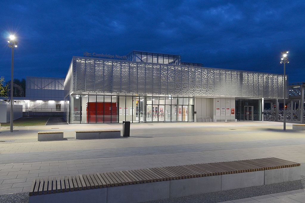
(Image by cmglee at wikipedia, licensed CC-SA)

Thsee patterns were described by the designers at Atkins (the contractors) like this:

The station is wrapped in three equal bands of aluminium panels which have been perforated with a design derived from John Horton Conway’s “Game of Life” theories which he established while at Gonville and Caius College, Cambridge in 1970. These beautiful, delicate panels ensure passive security to ground floor glazed areas, assist with wayfinding while crossing the footbridge and allow the building to transform its appearance between day and night through sensitive backlighting.

This quote is from the original article (archived here), but it's since been corrected, most probably in response to the anguished cries of thousands of Cambridge nerds who swiftly pointed out that, in fact, these patterns weren't Life as we know it, but were actually one-dimensional cellular automata, and so linked, not so much with Cambridge's John Horton Conway, as with noted Oxford/CalTech alumnus Stephen "Mr Mathematica" Wolfram.

I think the designers did a great job using these simple graphics to "create a harmonic relationship with the scientific research and industry of the Cambridge Colleges and nearby Science Park".

So what is a one-dimensional cellular automaton?

A cellular automaton is a mathematical model that creates patterns automatically according to simple rules. In its simplest, one-dimensional form, it's a row of empty squares, each of which can be occupied or empty. The rules for the model determine how sensitive the occupants of each square are to their immediate left and right neighbours, and whether, after some unspecified time, they survive or die. Sometimes empty squares can miraculously become occupied. Because a square has just two immediate neighbours, there are 8 different cases to consider, ranging from all empty ("□□□" or 000 in binary) to all full ("■■■" or 111).

The rule determines how one generation changes to the next by specifying the outcome for each of the 8 cases. So, for example, an empty square surrounded by empty neighbours can continue to be empty (false, or 0), or it can produce a new occupant in the next generation, (true, or 1). There are 256 different combinations, since each of the 8 cases can be either 0 or 1.

The wikipedia has this nice animation showing how the rule produces the next generation of squares.

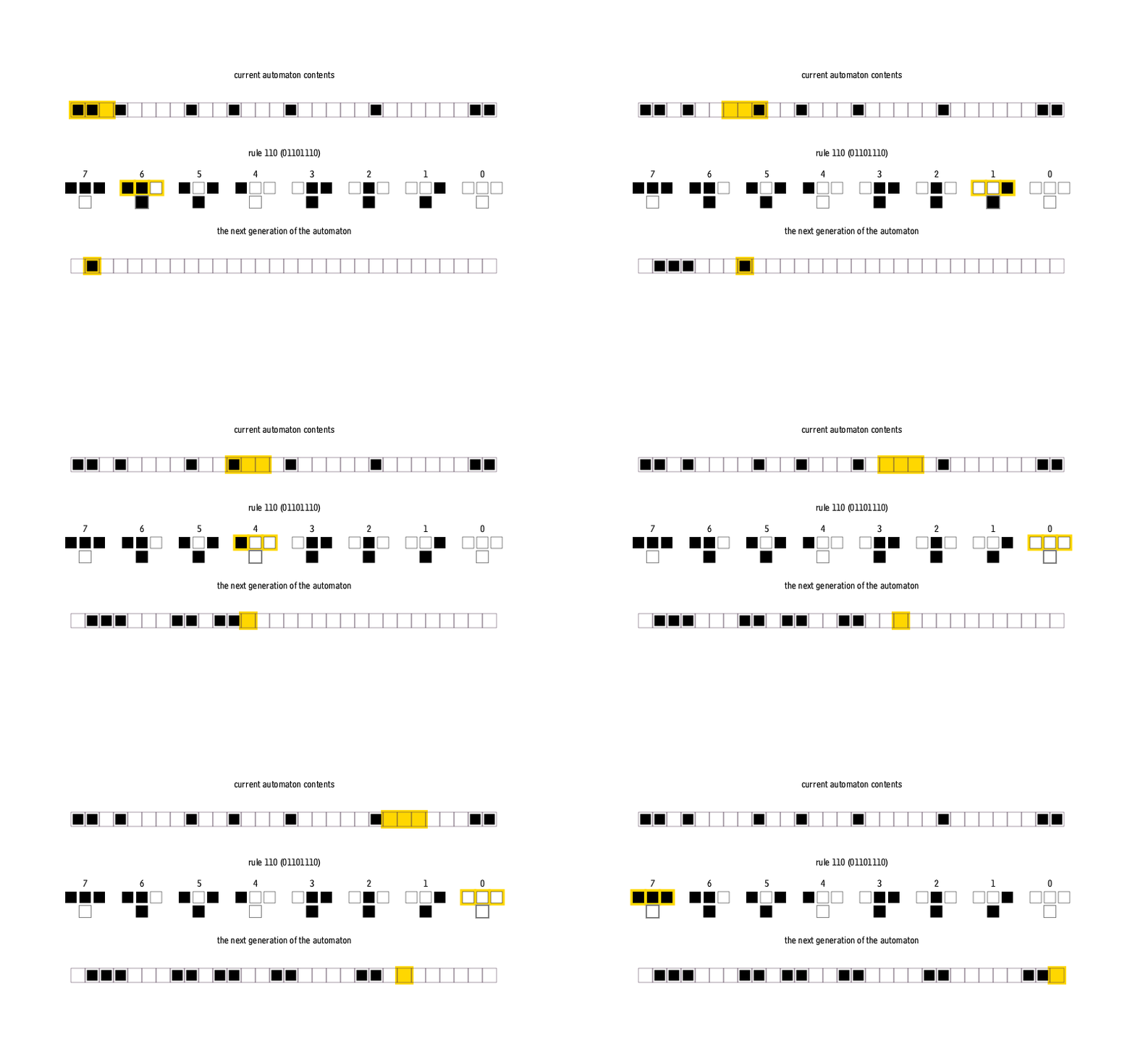
(Well, it has this nice animation now...)

First steps

To explore these simple automata, I started^[1] by making a Julia structure:

mutable struct CA
    rule::Int64
    cells::BitArray{1}
    colorstops::Array{Float64, 1}
    ruleset::BitArray{1}
    generation::Int64
    function CA(rule, ncells = 100)
        cells                    = falses(ncells)
        colorstops               = zeros(Float64, ncells)
        ruleset                  = binary_to_array(rule)
        cells[length(cells) ÷ 2] = true
        generation               = 1
        new(rule, cells, colorstops, ruleset, generation)
    end
end

The cells array can hold trues or falses. The colorstops array is eventually going to hold some color information. The middle cell is seeded with a single starter value.

The binary_to_array() function just converts a binary number to a bit array (I suspect there's a quicker way).

function binary_to_array(n)
    a = BitArray{1}()
    for c in 7:-1:0
        k = n >> c
        push!(a, (k & 1 == 1 ? true : false))
    end
    return a
end

The rules() function takes the values of an individual and its neighbours and applies the rule that determines its state for the next generation:

function rules(ca::CA, a, b, c)
    lng = length(ca.ruleset)
    return ca.ruleset[mod1(lng - (4a + 2b + c), lng)]
end

And a nextgeneration() function applies the rule to all the cells. I decided to make it wrap around, so that the final cell considers the first cell as one of its neighbours.

function nextgeneration(ca::CA)
    l = length(ca.cells)
    nextgen = falses(l)
    for i in 1:l
        left   = ca.cells[mod1(i - 1, l)]
        me     = ca.cells[mod1(i, l)]
        right  = ca.cells[mod1(i + 1, l)]
        nextgen[i] = rules(ca, left, me, right)
    end
    ca.cells = nextgen
    ca.generation += 1
    return ca
end

We'll also teach Julia how to show an automaton in the terminal:

Base.show(io::IO, ::MIME"text/plain", ca::CA) =
    print(io, join([c ? "■" : " " for c in ca.cells]))

So now we can create a cellular automaton by providing a rule number (using the default of 100 cells):

ca = CA(30)

update the automaton like this:

nextgeneration(ca)

and show a historical diagram of its evolution:

for i in 1:30
    display(nextgeneration(ca))
end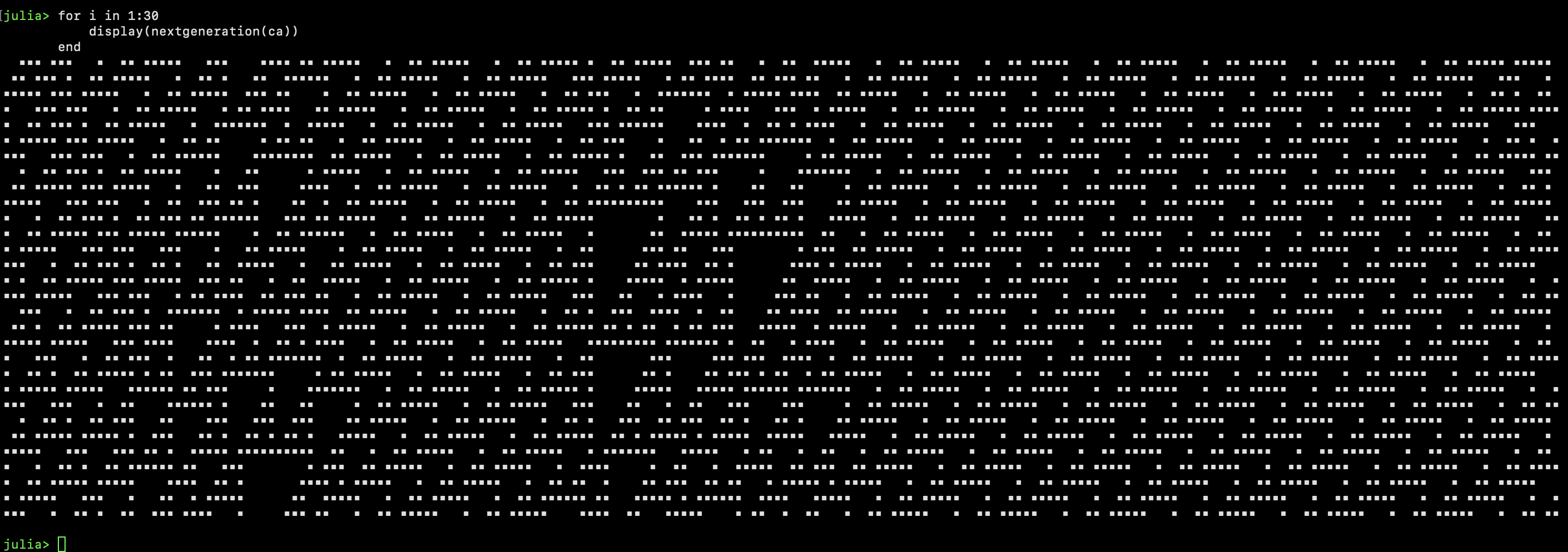

Some graphics

The REPL display is more or less functional, but I want to play with the graphic output, so (you guessed):

using Luxor, Colors

function draw(ca::CA, cellwidth=10)
    lng = length(ca.cells)
    for i in 1:lng
        if ca.cells[i] == true
            pt = Point(-(lng ÷ 2) * cellwidth + i * cellwidth, 0)
            box(pt, cellwidth, cellwidth, :fill)
        end
    end
end

@png begin
    ca = CA(30, 200)
    sidelength = 4
    # start at the top
    translate(boxtopcenter(BoundingBox()) + sidelength)
    for i in 1:200
        draw(ca, sidelength)
        nextgeneration(ca)
        translate(Point(0, sidelength))
    end
end 800 850 "../images/automata/simple-ca.png"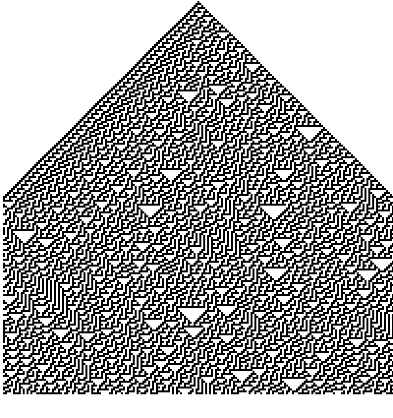

You can call nextgeneration() without displaying the results, of course. This lets you jump into the future history of an automaton at warp speed.

@png begin
    ca = CA(110, 200)
    translate(boxtopcenter(BoundingBox()) + sidelength)
    sidelength = 4
    # into the future
    for _ in 1:200_000
        nextgeneration(ca)
    end
    for _ in 1:195
        draw(ca, sidelength)
        nextgeneration(ca)
        translate(Point(0, sidelength))
    end
end 800 800 "../images/automata/simple-ca-future.png"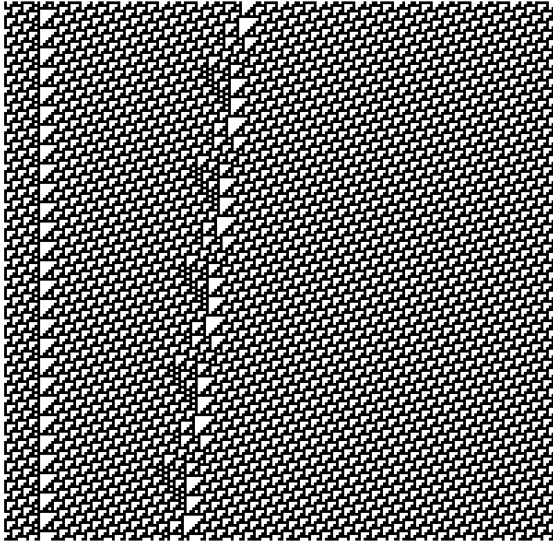

I found that sometimes drawing them from left to right looked better (like videos recorded on phones...?):

@png begin
    ca = CA(30)
    translate(boxmiddleleft(BoundingBox()) + sidelength)
    rotate(-π/2)
    sidelength = 3.5
    for i in 1:320
        draw(ca, sidelength)
        nextgeneration(ca)
        translate(Point(0, sidelength))
    end
end 1000 400 "../images/automata/simple-landscape-ca.png"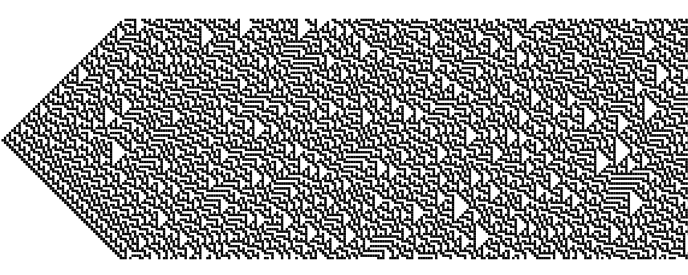

And now in color

So far I haven't used the color information that's stored.

The nextgeneration() function can be updated with instructions about how to modify the color of the next generation, based on the current set of three cells.

function nextgeneration(ca::CA)
    l = length(ca.cells)
    nextgen = falses(l)
    for i in 1:l
        left   = ca.cells[mod1(i - 1, l)]
        me     = ca.cells[mod1(i, l)]
        right  = ca.cells[mod1(i + 1, l)]
        nextgen[i] = rules(ca, left, me, right)
        if me == 1
            ca.colorstops[i] = mod(ca.colorstops[i] + 0.1, 1)
        elseif left == 1 && right == 1
            ca.colorstops[i] = mod(ca.colorstops[i] - 0.1, 1)
        else
            ca.colorstops[i] = 0
        end
    end
    ca.cells = nextgen
    ca.generation += 1
    return ca
end

and the draw() function can be adapted to make use of the color information. I decided to avoid tackling RGB color value transformations for a first pass, so the single value between 0 and 1 is used to select a color from a color map.

using ColorSchemes

function drawcolor(ca::CA, cellwidth=10;
        scheme=ColorSchemes.leonardo)
    lng = length(ca.cells)
    for i in 1:lng
        if ca.cells[i] == true
            sethue(get(scheme, ca.colorstops[i]))
            pt = Point(-(lng ÷ 2) * cellwidth + (i * cellwidth), 0)
            box(pt, cellwidth, cellwidth, :fill)
        end
    end
end

@svg begin
    background("darkorchid4")
    ca = CA(135, 65)
    # randomize start state
    ca.cells = rand(Bool, length(ca.cells))
    sidelength = 5
    translate(boxmiddleleft(BoundingBox()) + sidelength)
    rotate(-π/2)
    for i in 1:195
        drawcolor(ca, sidelength, scheme=ColorSchemes.cubehelix)
        nextgeneration(ca)
        translate(Point(0, sidelength))
    end
end 1000 400 "../images/automata/simple-color-ca.svg"

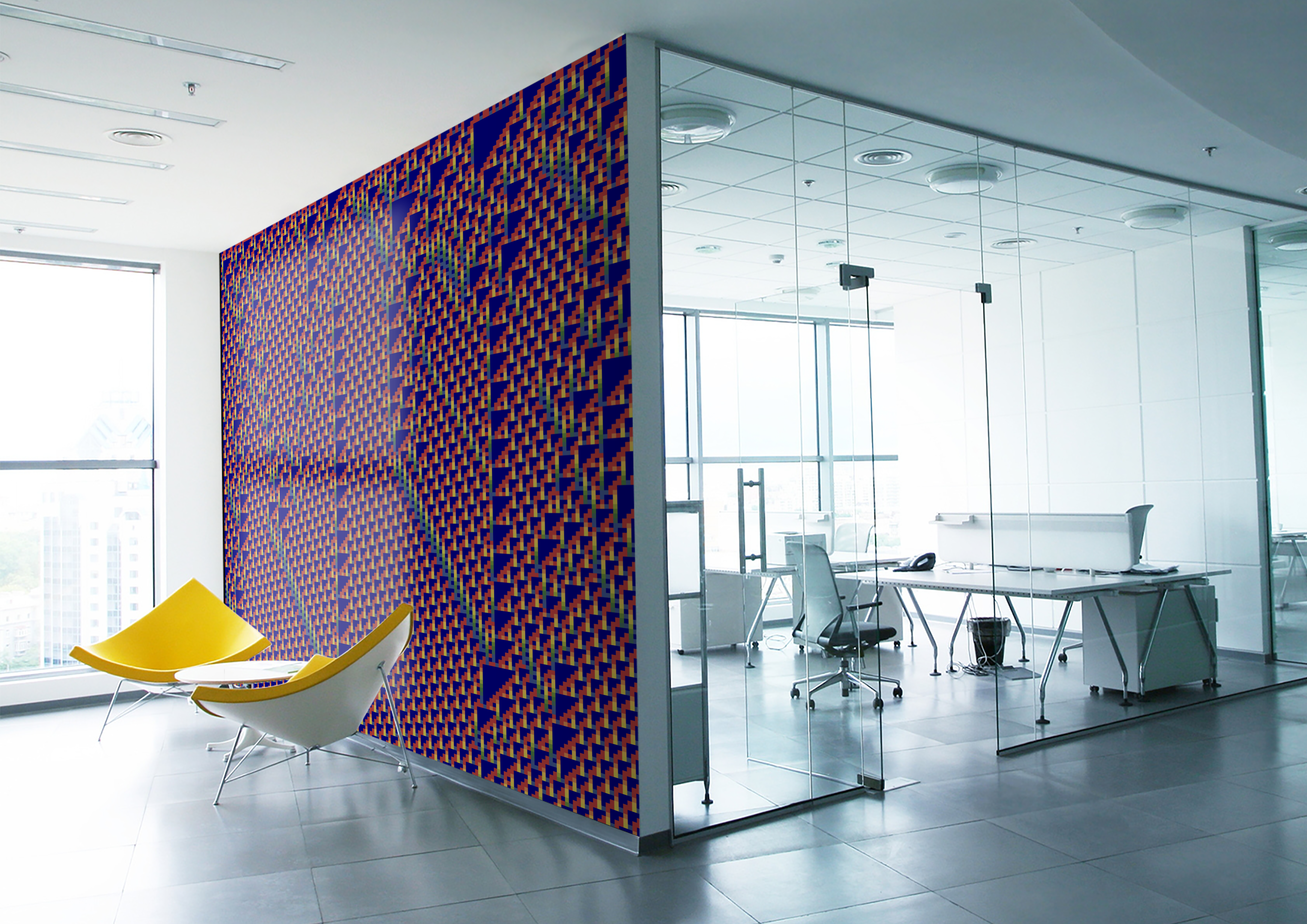
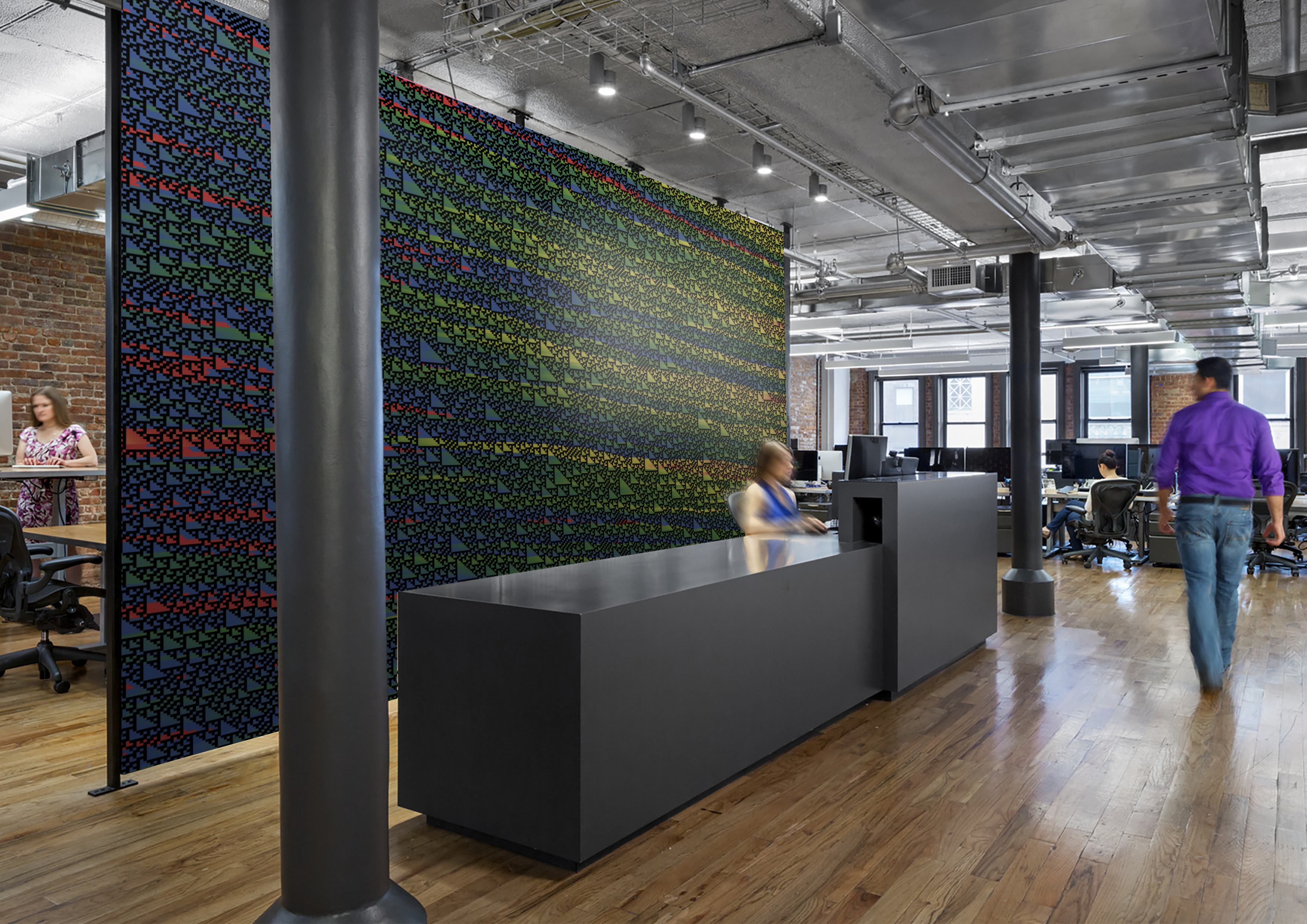
This could lead to hours of entertainment (depending on your definition of fun, of course). I uploaded a few experiments that didn't turn out too badly on Flickr. The current rules show a kind of literal winning streak, as a cell that remains occupied for many generations ends up being brightly illuminated.

I think these images look quite good when scaled up. It only takes about a second to draw these, but would take much longer to stick them on the wall:

The rules for specifying a change in color could do with some kind of systematic definition, perhaps, such that, say, "rule C81" means "increase colorstop by amount if previous parent is 1, decrease it if previous uncle-aunt is 1", and so on. Then you could pass a set of color rules to the drawing function. (uncle-aunt? I couldn't find a word for something that is either an uncle or an aunt, but not a parent...)

Instead of drawing simple squares, it's possible to draw other shapes. I'm quite fond of the squircle — you can change the rt parameter to get different shapes:

function drawcolorsquircle(ca::CA, cellwidth=10;
        scheme=ColorSchemes.leonardo)
    lng = length(ca.cells)
    for i in 1:lng
        if ca.cells[i] == true
            sethue(get(scheme, ca.colorstops[i]))
            pt = Point(-(lng ÷ 2) * cellwidth + (i * cellwidth), 0)
            squircle(pt, cellwidth, cellwidth, rt=6.0, :fill)
        end
    end
end

@svg begin
    background("navyblue")
    ca = CA(110, 30)
    # randomize start state
    ca.cells = rand(Bool, length(ca.cells))
    translate(boxmiddleleft(BoundingBox()) + sidelength)
    rotate(-π/2)
    sidelength = 10
    for i in 1:100
        drawcolorsquircle(ca, sidelength, scheme=ColorSchemes.Dark2_8)
        nextgeneration(ca)
        translate(Point(0, sidelength))
    end
end 1000 400 "../images/automata/simple-color-ca-squircle.svg"

(This SVG is quite big, and won't display in Juno. But it should load in a browser.)

Getting around to it

It occurred to me that you could take a rectangular array and wrap it into a circle.

function drawsector(ca::CA, cellwidth=10;
        scheme=ColorSchemes.leonardo,
        centralradius = 10)
    lng = length(ca.cells)
    width = lng * cellwidth
    angulargap = 2π/lng
    for i in 1:lng
        sethue(get(scheme, ca.colorstops[i]))
        innerradius = centralradius
        outerradius = centralradius + cellwidth
        startang    = rescale(i, 1, lng, 0, 2π)
        endang      = startang + angulargap
        if ca.cells[i] == true
            sector(O, innerradius, outerradius, startang, endang, :fillstroke)
        end
    end
end

function drawrule(rulenumber, pos)
    @layer begin
        translate(pos)
        sethue("black")
        text(string(rulenumber), halign=:center, valign=:middle)
        rotate(-π/2)
        ca = CA(rulenumber, 50)
        # randomize start state
        # ca.cells = rand(Bool, length(ca.cells))
        sidelength = 2
        setline(0.0)
        for n in 5:sidelength:30
            drawsector(ca, sidelength,
            scheme=ColorSchemes.klimt,
            centralradius = n)
            nextgeneration(ca)
        end
    end
end

This shows all the rules in this circular form.

let
    # best in SVG or PDF, but PNG is faster
    Drawing(1200, 1200, "../images/automata/color-sector-assembly.svg")
    origin()
    background("azure")
    fontsize(8)
    for (pos, n) in Tiler(1200, 1200, 16, 16)
        drawrule(n-1, pos)
    end
    finish()
    preview()
end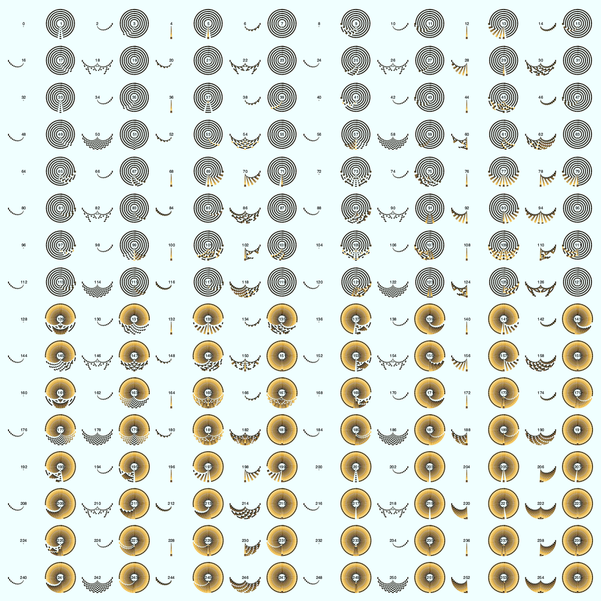

(PNG shown here. This image is quite demanding for SVG and can take a while to load, even though it doesn't take long to generate.)

After playing with this idea, I thought it would make some nice jewellery:

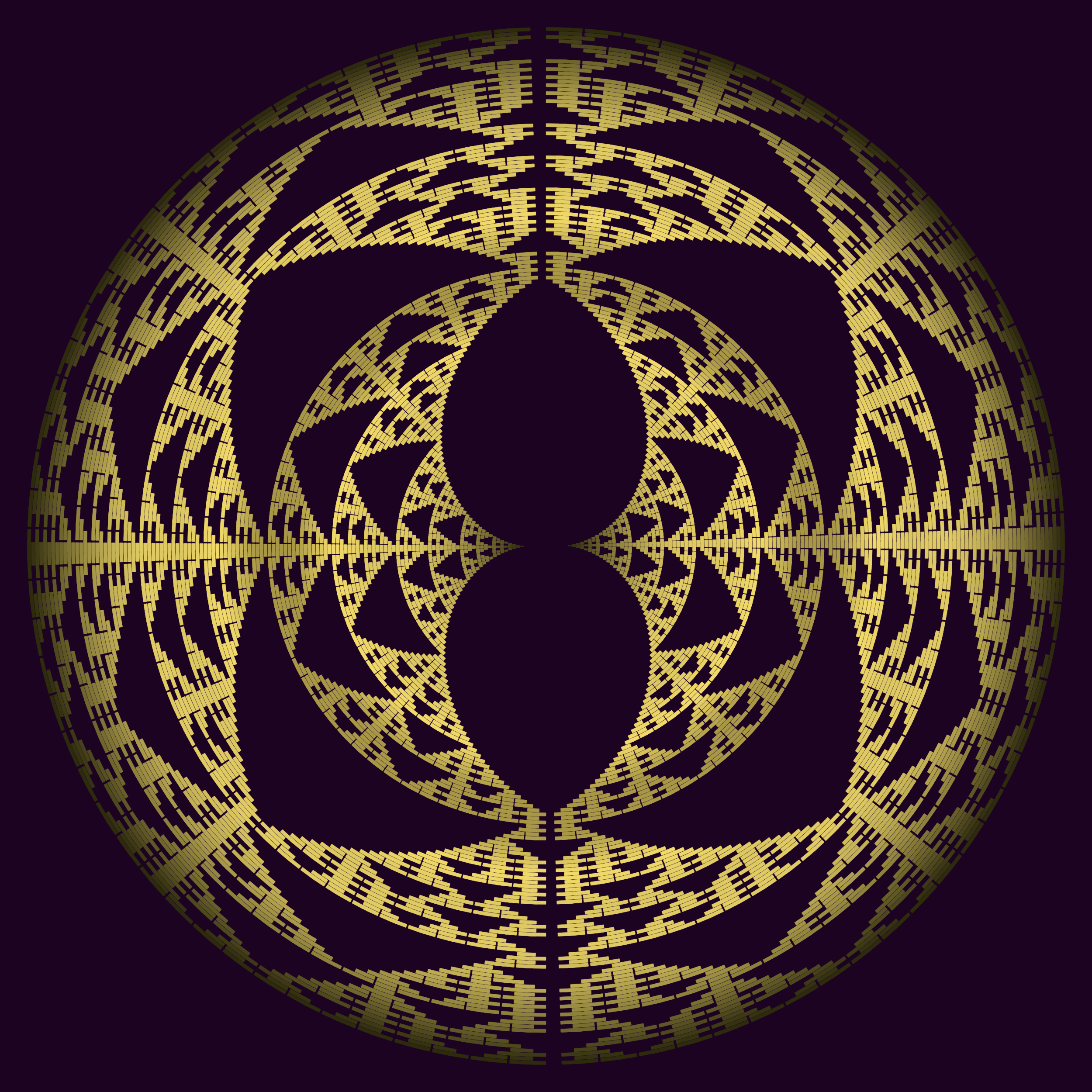
This is rule 150. I mapped the array to a semicircle and drew it twice.

And it moves

Many of the rules have limited career paths. Some fizzle out very quickly, others settle down into a stable if repetitive life style. There are a few that continue to make patterns as the number of generations heads off into the thousands.

The unpredictable high achiever of the 1D cellular automata world is Rule 110. The rule itself is so simple, it could have been described in a Shakespeare play:

[Enter HAMLET, stage left.]
For Zeros become Ones at all positions,
Where the value to the right is One.
Yet Ones are changed to Zeros where'er
The values to left and right are One.

And yet this simple rule has been the subject of an astonishing amount of analysis, such as this in-depth paper by Martinez et al published in the wonderfully-named International Journal of Unconventional Computing. Matthew Cook's famous paper proved that Rule 110 is capable of emulating the activity of a Turing machine.

I understood very little of those wonderful papers, but they did make me want to at least see Rule 110 in action, just in case I could spot all those cyclic tags, meta-gliders, and pseudo-solitons.

function frame(scene, framenumber, ca, cahistory, sidelength;
            smoothscrolling=10)
    background(colorant"navy")
    fontsize(12)
    sethue(colorant"azure")
    text(string(ca.generation), boxtopright(BoundingBox()) + (-30, 20),
        halign=:right)
    setline(0.1)

    # get in position for the first row
    translate(boxmiddleleft(BoundingBox()))
    rotate(-π/2)

    # for smooth scrolling
    translate(0, -(mod1(framenumber, smoothscrolling))
        * sidelength/smoothscrolling)

    lng = length(ca.cells)
    for gen in cahistory
        for (n, cell) in enumerate(gen)
            if cell == true
                pt = Point(-(lng / 2) * sidelength + (n * sidelength), 0)
                box(pt, sidelength - 2, sidelength - 2, :fill)
            end
        end
        translate(Point(0, sidelength))
    end
    # "beautiful buttery scrolling"
    if framenumber % smoothscrolling == 0
        # drop oldest, add a new generation
        popfirst!(cahistory)
        nextgeneration(ca)
        push!(cahistory, ca.cells)
    end
end

function makeanimation(rule, filename)
    width, height = (1920, 1080)
    sidelength = 6
    cellularmovie = Movie(width, height, "cellularmovie")
    ca = CA(rule, convert(Int, height÷sidelength))
    cahistory = []
    # initial
    for _ in 1:width÷sidelength
        push!(cahistory, ca.cells)
        nextgeneration(ca)
    end
    animate(cellularmovie,
        [Scene(cellularmovie, (s, f) ->
            frame(s, f, ca, cahistory, sidelength, smoothscrolling=4),
                1:500)],
    createmovie=true,
    pathname="$(filename)")
end

makeanimation(110, "../images/automata/animated-cellular-automaton")

If each frame moved the history 'window' by one generation, you'd get a jerky animation. The smooth-scrolling used here shifts the contents by a few pixels in each frame but changes the contents less often. This requires more frames than generations, so 300 frames with a smoothscrolling value of 10 shows only 30 new generations after the initial bunch.

This GIF does have a few problems; the conflicting demands of file size, image size, image quality, and scroll speed work against each other. There's a slight flickering, due I think to the rounding or aliasing in the GIF. You could make the GIF as long as you want, subject of course to the maximum size of animated GIF that you're prepared to handle. (And yes, this page does take a long time to load. Sorry.)

Videos also have their problems with this kind of content, because the downsampling commonly applied can affect the detail. To see what I mean, try watching Rule 110: The Movie (on YouTube). (This is my submission for YouTube's Most Boring Video 2018 competition.)

Solid work

If you want to do more than just look at pictures on the screen—perhaps you're building your own railway station?—here are some tips for exporting the graphics to your favourite 3D modeller.

First, place a box or shape around the outside of the design, and use the :path action rather than :fill or :stroke. Then, to draw what are now the 'holes', use newsubpath() before drawing each hole, and make sure to draw the holes with reversed paths (using the reversepath keyword, for example).

function drawaspath(ca::CA;
        cellwidth=10)
    lng = length(ca.cells)
    for i in 1:lng
        if ca.cells[i] == true
            newsubpath()
            pt = Point(-(lng ÷ 2) * cellwidth + (i * cellwidth), 0)
            poly(box(pt, cellwidth - 2, cellwidth - 2, vertices=true),
                :path, reversepath=true, close=true)
        end
    end
end

@svg begin
    background("black")
    ca = CA(110, 40)
    ca.cells = rand(Bool, length(ca.cells))
    cellwidth = 7
    bxw = boxwidth(BoundingBox() * 0.98)/2
    squircle(O, bxw, bxw, rt=0.1, :path)
    translate(boxtopcenter(BoundingBox()) + (-5, 7))
    for i in 1:40
        translate(0, cellwidth)
        drawaspath(ca, cellwidth=cellwidth)
        nextgeneration(ca)
    end
    sethue("grey80")
    fillpath()
end 300 300 "../images/automata/ca-as-path.svg"

So this is a single path, and the holes are reversed subpaths. When you import this single path into a 3D modelling program, you should be able to extrude it into a solid without problems. Here's one modelled as a thin gold reflective sheet.

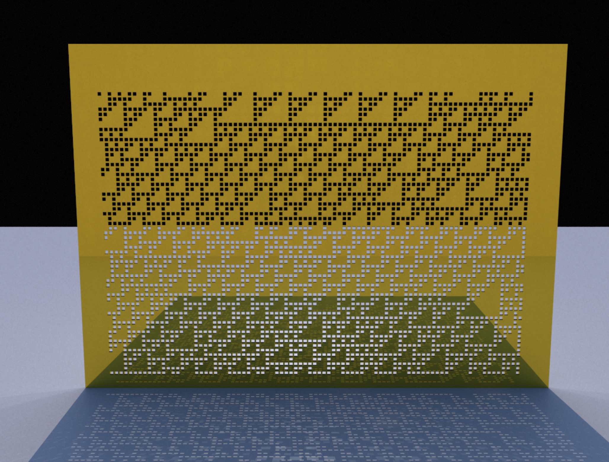
It's hard to resist playing with 3D modellers... I added some fog and a rusty metal effect:

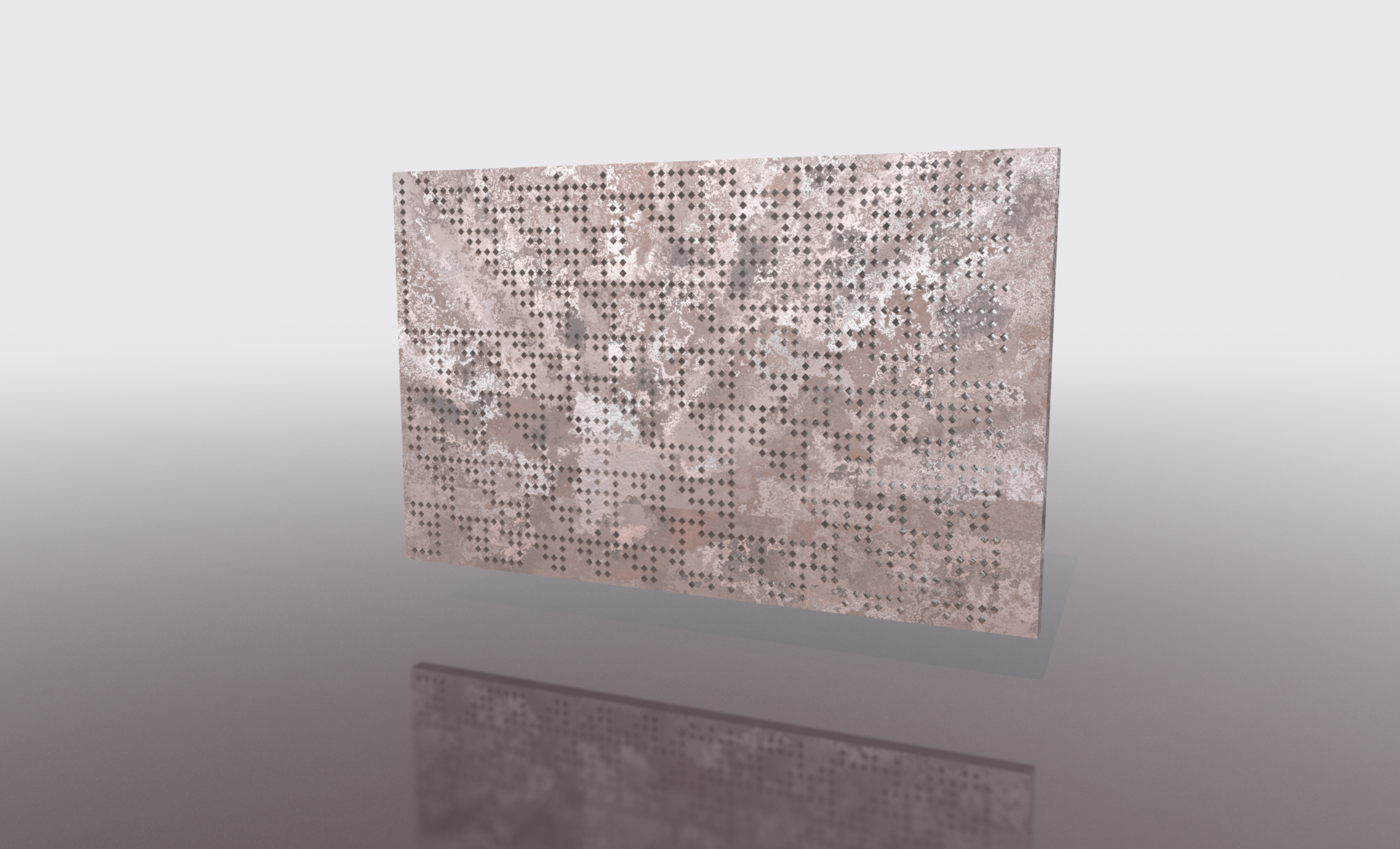
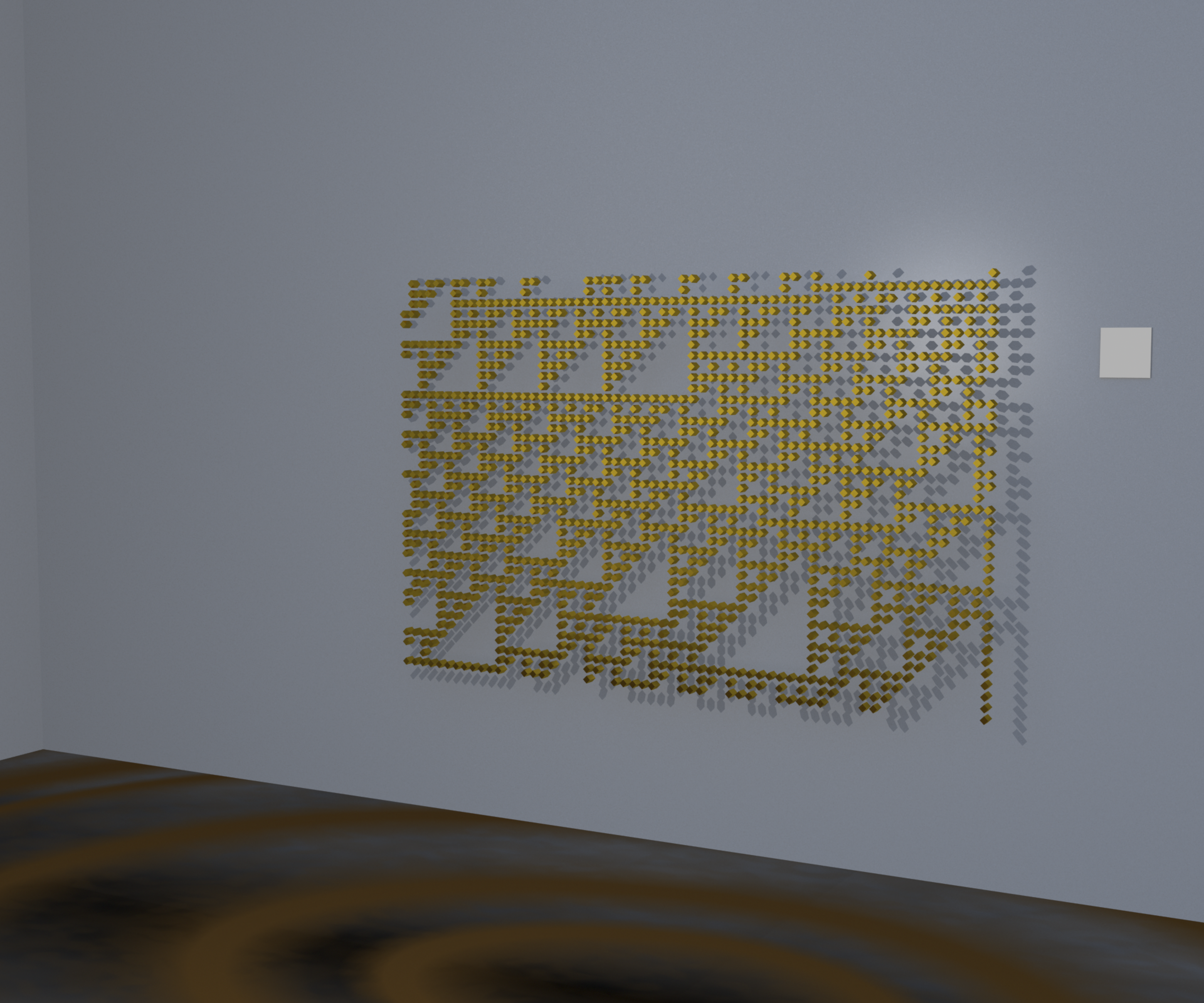
If you omit the surrounding path, it might still work visually. It would be a challenge to hang all these pieces on a gallery wall:

These little critters are quite interesting, and there are a fair number of scientific papers with "cellular automata" in the title . I think this must be because, although things don't get much simpler than a cellular automaton, perhaps they might—in some strange way—be similar to how the universe itself works when you zoom in close enough.

[2018-11-29]

[1]	At the time of writing this I couldn't find any working Julia packages that did one-dimensional cellular automata. But if I had found one, I probably wouldn't have written any of the above anyway.

This page was generated using Literate.jl.