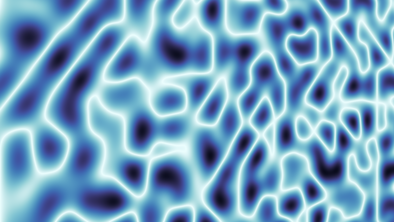
Noise

This is another post in the ongoing series in which I try to learn 2D vector graphics using Julia. It doesn't contain any revelations or new material, and you should visit the following sites if you're looking for a good introduction to the subject of noise in graphics:

• red blob games

• adrianbiagioli

• khan academy

I'm using Julia version 1.0 if you want to play along; you can find the source files and notebooks on the github. If you do, you'll need the packages Luxor, Colors, and ColorSchemes. I used Literate.jl to produce the Markdown and Jupyter notebook versions.

Random versus Noise

Luxor provides a function called noise(). This can accept a single floating-point number as input, and it returns a value between 0.0 and 1.0.

using Luxor

noise(0.0)
0.8261106995884773

noise(1.0)
0.5

noise(2.0)
0.4460609053497945

It will be easier to draw some graphs. Here's a quick throwaway function to draw a simple graph.

function graph(a, width = 800;
        startnumber     = 0,
        endnumber       = 1,
        style           = :line,
        margin          = 30)
    setline(1)
    bars(a, labels      =false,
            xwidth      = (width - 2margin)/length(a),
            yheight     =40,
            barfunction = (bottom::Point, top::Point, value;
        extremes=extrema(a), barnumber=0, bartotal=0) ->
            begin
                if style == :line
                    line(bottom, top, :stroke)
                else
                    circle(top, 1, :fill)
                end
            end)
    sethue("black")
    label(string(startnumber), :S,
        Point(0, 0), offset=10)
    label(string(endnumber), :S,
        Point(width - 2margin, 0), offset=10)
end

function drawgraph(startvalue, endvalue, filename)
    Drawing(800, 150, filename)
    background("white")
    origin()
    # move to top left corner
    margin=30
    translate(BoundingBox()[1] + (margin, boxheight(BoundingBox()/2)))
    sethue("black")
    graph(noise.(range(startvalue, endvalue, length=200)),
        startnumber=startvalue,
        endnumber=endvalue)
    finish(); preview()
end

To test this out, graph 200 random integers:

Drawing(800, 150, "images/noise/graph-random.png")
background("white")
origin() ## move to top left corner
margin=30
translate(BoundingBox()[1] + (margin, boxheight(BoundingBox()/2)))
sethue("black")
graph(rand(200))
finish(); preview()

To start with, let's graph the output of the noise() function for the first 200 integers:

drawgraph(0, 200, "images/noise/graph-0-200.png")

It looks very random. But let's look at 200 values between 0 and 10:

drawgraph(0, 10, "images/noise/graph-0-10.png")

There's some randomness, but it's smoother, and looks more natural.

Zoom and enhance, between 0 and 5:

drawgraph(0, 5, "images/noise/graph-5.png")

You can see that the left half of the 0 to 10 graph has been stretched.

Between 0 and 1:

drawgraph(0, 1, "images/noise/graph-0-1.png")

One more for luck:

drawgraph(0, 0.5, "images/noise/graph-0-05.png")

The more often you sample the noise space (ie the shorter the gaps between the set of values passed to noise(), the closer together the output values will be.

So the noise() function provides gently changing undulations rather than the unpredictable jumps of randomness. Here's a slowly changing color pattern in the LCHab color space, using a set of noisy values to choose the hue. We'll change the length of each line as well just for fun:

using Colors
@svg begin  ## switch to SVG for better graphic quality
    rate = .009
    setline(2)
    for x in -250:2:250
        yn = noise(x * rate)
        hue = rescale(yn, 0, 1, 0, 359)
        sethue(LCHab(50, 100, hue))
        ht = rescale(yn, 0, 1, 10, 100)
        line(Point(x, -ht/2), Point(x, ht/2), :stroke)
    end
end 600 200 "images/noise/colorbars.svg"

You can use noisy values to specify other changing parameters. For example, let's place some pebbles at random, and control their size using a noisy distribution, to give the illusion of a naturally changing distribution.

function drawpebble(pt, radius)
    sethue("grey60")
    @layer begin
        transform([rand(0.5:0.1:1) 0 0 rand(0.5:0.1:1) 0 0])
        circle(pt, radius, :fill)
        for i in 1:-0.02:0.2
            sethue(rescale(i, 1, 0,   0.5 + rand(0:0.1:0.3), 1.0),
                   rescale(i, 1, 0.1, 0.4 + rand(0:0.1:0.5), 1.0),
                   rescale(i, 1, 0.3, 0.5, 1.0))
            setopacity(1 - i)
            circle(pt + (-2i, -2i), i * radius, :fill)
        end
    end
end


@png begin
    # switch to PNG, SVG can't handle this
    background("palegoldenrod")
    pebblesize = 12
    for i in 1:6000
        pt = Point(rand(-400:400), rand(-200:200))
        n = noise(pt.x * 0.002)
        drawpebble(pt, pebblesize * n)
    end
end 800 400 "images/noise/pebbles.png"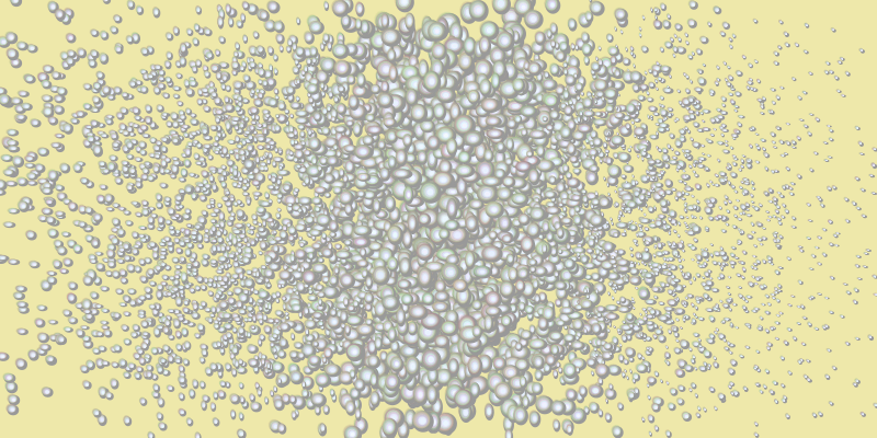

Detail and persistence

The noise() function has two optional keyword arguments that let you tweak the knobs of the noise generator.

The first is detail, an integer. Increasing it from the default value of 1 upwards will add finer detail to the basic noise. The second is persistence, a floating-point value between 0 and 1 (or more).

detail is graphed here with values from 1 to 12. As the level increases, you can see that the same overall noise contours are gradually modulated with finer variations.

function detailgraph()
    @svg begin
        margin=30
        translate(BoundingBox()[1] + (margin, 0))
        setline(.5)
        sethue("black")
        stopat = 2
        r = range(0, length=400, stop=stopat)
        for detail in 1:2:12
            translate(0, 100)
            sethue("red")
            graph(noise.(r), style=:circle, endnumber=stopat)
            sethue("black")
            text("detail = $detail, persistence = 0.9", Point(200, 15))
            graph(noise.(r, detail=detail, persistence=0.9), endnumber=stopat)
        end
    end 800 650 "images/noise/detail-graph.svg"
 end
detailgraph()

You can see the original noisy curve (in red) behind each more detailed graph. The noise generator is doubling the frequency but halving the amplitude every time you go one level higher. Noise, like music, can have octaves of higher frequencies mixed with lower fundamental frequency. The detail keyword is adding one or more octaves of noise.

The persistence argument defaults to zero. The value controls the amplitude of each successive octave of noise, with higher values of persistence producing higher levels of finer detail, as the values persist for longer.

function persistencegraph()
    @svg begin
        setline(.5)
        sethue("black")
        margin=30
        translate(BoundingBox()[1] + (margin, 0))
        stopat = 10
        r = range(0, length=400, stop=stopat)
        for p in 0:0.25:2
            translate(0, 70)
            sethue("red")
            graph(noise.(r, detail=4, persistence=0),
                endnumber=stopat, style=:circle)
            sethue("black")
            text("detail = 4, persistence = $p", Point(200, 15))
            graph(noise.(r, detail=4, persistence=p),
                endnumber=stopat)
        end
    end 800 675 "images/noise/persistence-graph.svg"
end

persistencegraph()

Here, the detail is kept at 4, and the persistence varies from 0 upwards. As the persistence increases, the effects accumulate, until the original curve is barely visible.

There are many uses for noisy input, such as generating varying shapes that don't have that undesirable 'too random' quality.

using ColorSchemes

function treerings()
    @svg begin
        nrate = 0.01
        npoints= 500
        nrings = 400
        rad = 20
        setline(0.5)
        for ring in nrings:-5:1
            pts = Point[]
            for i in 1:npoints
                push!(pts, polar(rad + (ring * noise(i * nrate)),
                    rescale(i, 1, npoints, 0, 2pi)))
            end
            sethue(get(ColorSchemes.sienna, noise(ring * 5nrate)))
            poly(pts, :fill, close=false)
            sethue("black")
            poly(pts, :stroke, close=false)
        end
    end 800 800 "images/noise/treerings.svg"
end

treerings()

Here's a more questionable idea, using noise to control the setting of a line of text.

function drawtextline(t, point, fsize; rate=0.1)
    for (n, c) in enumerate(split(t, ""))
        f = fsize * noise(n * rate, persistence=0, detail=4)
        fontsize(f)
        te = textextents(c)
        text(c, point)
        point = Point(point.x + te[5] * 0.98, 0) ## tightness is tight
        move(point)
    end
end

@png begin
    fontface("Bodoni")
    drawtextline("variablefontsizetextsettingiscool,orisit?",
        O - (380, 0), 50, rate=.11)
end 800 120 "images/noise/text-setting.png"

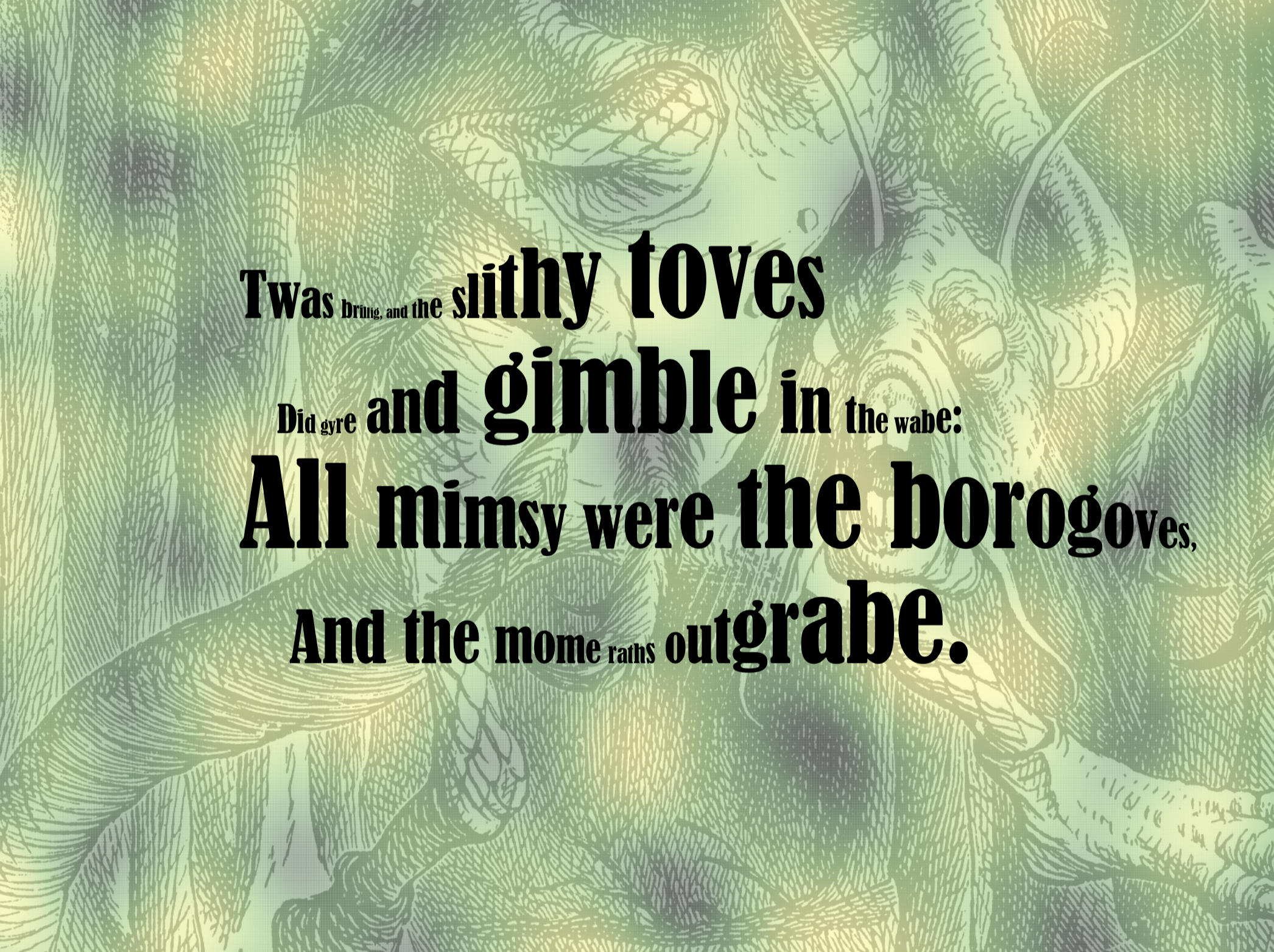
I then used the readpng() and placeimage() functions to add a background image (the original Tenniel illustration), with the following result:

Why noise?

The first use of computer graphics in movies is generally considered to be Tron (1981).

Tron lies at the very beginning of the history of CGI in the movies, and the technology available to the artists, mathematicians, and programmers making Tron was amazingly underpowered compared with the computing power that we have today on our wrists, let alone on our phones.

Ken Perlin was a mathematician and programmer who worked on Tron, and (I think after the film was released) he realised that there was room for using mathematical techniques for realistic-looking surfaces and textures, such as terrain.

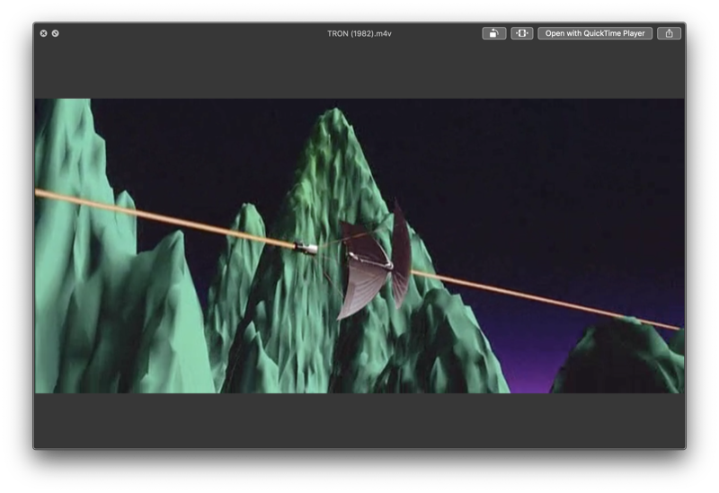
Ken's noise, or Perlin Noise as it became known, was quickly adodpted as the best way to generate naturalistic surfaces.

I think the reason why natural scenes appear to us as variable but not completely random is due to the (possibly hidden) larger scale processes that make smaller and more visible details clump together, and appear to work together and change gradually. For example, clouds, mountains, and pebble beaches have large scale structure controlled by unseen forces like heat, pressure, and gravity. We mostly see the objects that are subject to these forces, rather than the forces themselves.

Moving into 2D

So far the noise we've been producing has been one-dimensional, although we've been using 2D graphics to draw it.

The noise() function can accept two floating-point numbers as input. These effectively define a rectangular grid of varying noise values: the x and y inputs produce a third value which requires representation.

A simple way of doing this is to draw a table and vary the color of each square, giving a type of heat map.

using ColorSchemes

@svg begin
    nrows = 40
    ncols = 40
    cellwidth = 15
    cellheight = 15
    table = Table(nrows, ncols, cellwidth, cellheight)
    rate = 0.1
    fontsize(5)
    for row in 1:nrows
        for col in 1:ncols
            zvalue = noise(row * rate, col * rate)
            sethue(get(ColorSchemes.temperaturemap, zvalue))
            box(table[row, col], table.colwidths[1], table.rowheights[1], :fill)
            sethue("black")
            text(string(round(zvalue, digits=1)), table[row, col], halign=:center, valign=:middle)
        end
    end
end 800 700 "images/noise/table.svg"

Alternatively, we can create a 3D surface and use the noise values for the height at each point. Normally this would require a visit to Julia's colorful and generally awesome Swedish-nightclub-themed Package manager, Pkg:

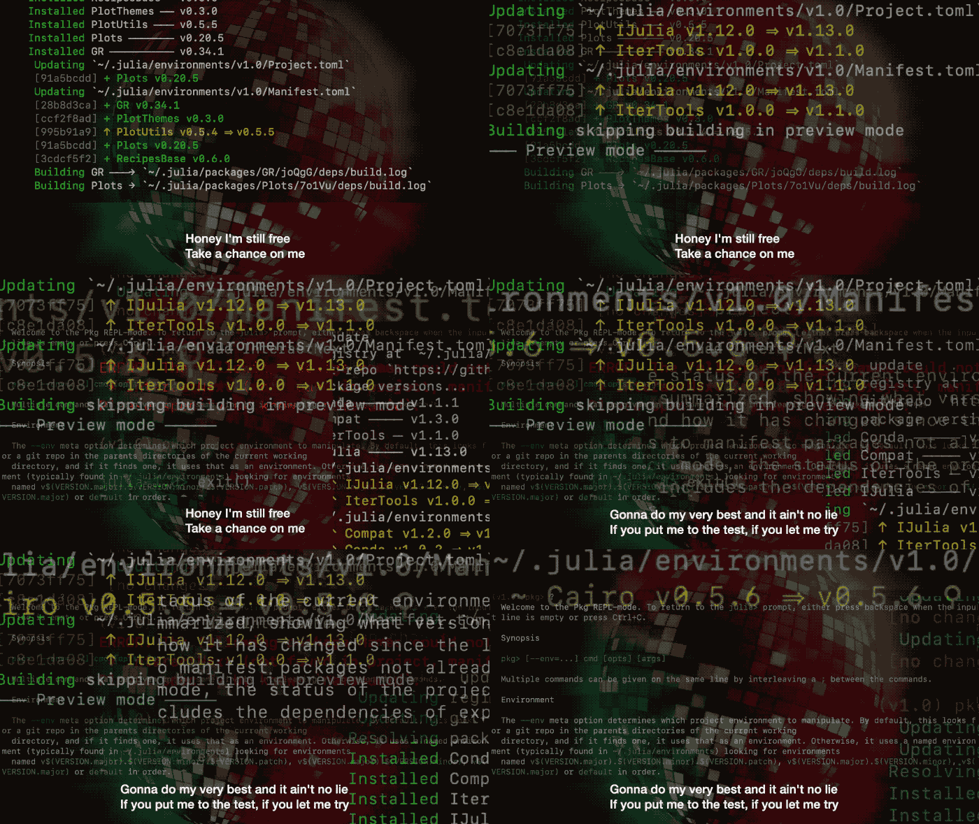
to download some of the cool plotting packages available, not least Simon Danisch's impressive Makie.jl.

But, just to be contrary, I decided to whip up a simple isometric projection:

function project(x, y, z;
        scalingfactor = 3, heightmultiplier = -1)
    # negative because y is positive downwards!
    u = (x - y)/sqrt(2)
    v = (x + 2(heightmultiplier * z) + y)/sqrt(6)
    return Point(scalingfactor * u, scalingfactor * v)
end

project(t; kwargs...) = project(t[1], t[2], t[3]; kwargs...)

function generatenoisearray(sx=100, sy=100;
    rate=0.5,
    detail=1,
    persistence=0)
    a = Array{Float64}(undef, sx, sy)
    for x in 1:sx
        for y in 1:sy
            a[x, y] = noise(x * rate, y * rate,
                detail=detail, persistence=persistence)
        end
    end
    return a
end

function isograph(a)
    @svg begin
        background("grey30")
        translate(0, -300)
        setline(0.5)
        sx, sy = size(a)
        scalingfactor = 5
        heightmultiplier = -6
        for x in 1:sx-1
            newpath()
            move(project(x, sy, -10,
                    scalingfactor = scalingfactor,
                    heightmultiplier = heightmultiplier))
            for y in sy-1:-1:1
                toppolygon = project.([
                    (x,     y,     a[x, y]),
                    (x + 1, y,     a[x + 1, y]),
                    (x + 1, y + 1, a[x + 1, y + 1]),
                    (x,     y + 1, a[x, y + 1])],
                        scalingfactor = scalingfactor,
                        heightmultiplier = heightmultiplier)
                centroid = polycentroid(toppolygon)
                line(centroid)
            end
            line(project(x, 1, -10,
                scalingfactor = scalingfactor,
                heightmultiplier = heightmultiplier))
            sethue("grey20")
            fillpreserve()
            sethue("grey85")
            strokepath()
        end
    end 800 700 "images/noise/isograph.svg"
end

isograph(generatenoisearray(80, 80, rate=0.08))

(This image reminds me of the famous Joy Division LP cover and T-shirt image, which features plots of the first ever pulsar discovered by Jocelyn Bell Burnell and Antony Hewish in 1967. This then became the basis of many entertaining blog posts, such as this one.)

A more conventional surface rendering is also possible:

function isograph(a)
    @png begin
        background("grey20")
        translate(0, -200)
        setline(0.5)
        sx, sy = size(a)
        for x in 1:sx-1
            for y in sy-1:-1:1
                toppolygon = project.([
                    (x,     y,     a[x, y]),
                    (x + 1, y,     a[x + 1, y]),
                    (x + 1, y + 1, a[x + 1, y + 1]),
                    (x,     y + 1, a[x, y + 1])],
                        heightmultiplier=-10,
                        scalingfactor=5)
                sethue("black")
                poly(toppolygon, close=true, :stroke)
                sethue(get(ColorSchemes.inferno, a[x, y]))
                poly(toppolygon, close=true, :fill)
            end
        end
    end 800 500 "images/noise/isosurface-2.png"
end

isograph(generatenoisearray(100, 100, rate=0.08))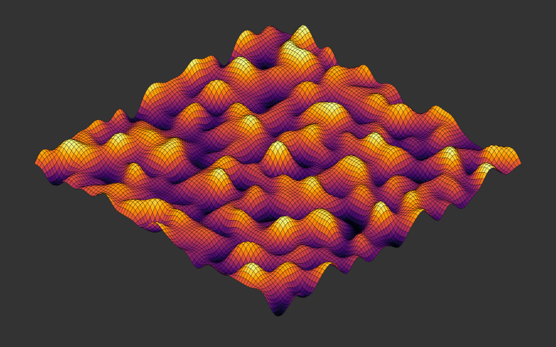

What, more dimensions?

So far we've been generating 2D noise. The noise() function can also accept three floating-point numbers as input. This produces noise values in 3D space, where each 3D point can have a noise value between 0 and 1. Rendering these point clouds is definitely a job for something other than a simple 2D graphics system. But, while we're here, let's have a go:

function buildarray(a::AbstractArray; rate=20)
    sx, sy, sz = size(a)
    for x in 1:sx
        for y in 1:sy
            for z in 1:sz
                a[x, y, z] = noise(x * rate, y * rate, z * rate)
            end
        end
    end
    return a
end

function iso3d(a)
    background("grey20")
    sethue("gray80")
    setline(0.15)
    rule.([Point(0, y) for y in -400:10:400])
    sx, sy, sz = size(a)
    for x in 1:sx
        for y in 1:sy
            for z in 1:sz
                noisevalue = a[x, y, z]
                sethue(get(ColorSchemes.plasma, noisevalue))
                pt = project(x, y, z, scalingfactor=8)
                setopacity(noisevalue)
                circle(pt, rescale(noisevalue, 0, 1, 0.05, 6), :fill)
            end
        end
    end
end

const A = Array{Float64, 3}(undef, 50, 50, 50)

@png begin
    iso3d(buildarray(A, rate=0.05))
end 800 800 "images/noise/isosolid.png"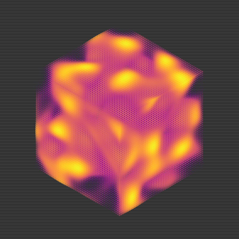

The noise values nearer 1 look like hot plasma, whereas values nearer 0 are almost translucent. It suggests what you might expect to see from a real volume visualization tool.

Journey to Algorithmia

The final images in this post combine 2D noise and 1D noise; 2D noise for the sky, and 1D noise to create the contours.

There's an initnoise() function. This is broadly the equivalent of the Random.seed!() function in Julia. This is useful when you want the noise to vary from image to image.

function layer(leftminheight, rightminheight, noiserate;
        detail=1, persistence=0)
    c1, c2, c3, c4 = box(BoundingBox(), vertices=true)
    ip1 = between(c1, c2, leftminheight)
    ip2 = between(c4, c3, rightminheight)
    topedge = Point[]
    initnoise(rand(1:12))
    for x in ip1.x:2:ip2.x
        ypos = between(ip1, ip2, rescale(x, ip1.x, ip2.x, 0, 1)).y
        ypos *= noise(x/noiserate, detail=detail, persistence=persistence)
        push!(topedge, Point(x, ypos))
    end
    p = [c1, topedge..., c4]
    poly(p, :fill, close=true)
end

function clouds()
    tiles = Tiler(boxwidth(BoundingBox()),
                  boxheight(BoundingBox()),
                  800, 800, margin=0)
    @layer begin
        transform([3 0 0 1 0 0])
        setopacity(0.3)
        noiserate = 0.03
        for (pos, n) in tiles
            nv = noise(pos.x * noiserate,
                       pos.y * noiserate,
                    detail=4, persistence=.4)
            setgray(nv)
            box(pos, tiles.tilewidth, tiles.tileheight, :fill)
        end
    end
end

function colorblend(fromcolor, tocolor, n=0.5)
    f = clamp(n, 0, 1)
    nc1 = convert(RGBA, fromcolor)
    nc2 = convert(RGBA, tocolor)
    from📕, from📗, from📘, from💡 =
        convert.(Float64, (nc1.r, nc1.g, nc1.b, nc1.alpha))
    to📕, to📗, to📘, to💡 =
        convert.(Float64, (nc2.r, nc2.g, nc2.b, nc1.alpha))
    new📕 = (f * (to📕 - from📕)) + from📕
    new📗 = (f * (to📗 - from📗)) + from📗
    new📘 = (f * (to📘 - from📘)) + from📘
    new💡 = (f * (to💡 - from💡)) + from💡
    return RGBA(new📕, new📗, new📘, new💡)
end

function landscape(scheme, filename)
    Drawing(800, 300, "$(filename).png")
    origin()
    # sky is gradient mesh
    bb = BoundingBox()
    mesh1 = mesh(box(bb, vertices=true), [
      get(scheme, rand()),
      get(scheme, rand()),
      get(scheme, rand()),
      get(scheme, rand())
      ])
    setmesh(mesh1)
    box(bb, :fill)
    # clouds are 2D noise
    clouds()
    # the sun is a disk placed at random
    @layer begin
        setopacity(0.25)
        sethue(get(scheme, .95))
        sunposition = boxtop(bb) +
            (rand(-boxwidth(bb)/3:boxwidth(bb)/3), boxheight(bb)/10)
        circle(sunposition, boxdiagonal(bb)/30, :fill)
    end
    setopacity(0.8)
    # how many layers
    len = 6
    noiselevels =  range(100, length=len, stop=10)
    detaillevels = 1:len
    persistencelevels = range(0.5, length=len, stop=0.95 )
    for (n, i) in enumerate(range(1, length=len, stop=0))
        # avoid extremes of range
        sethue(colorblend(get(scheme, .05), get(scheme, .95), i))
        layer(i - rand()/2, i - rand()/2,
            noiselevels[n], detail=detaillevels[n],
            persistence=persistencelevels[n])
    end
    finish()
    preview()
end

landscape(ColorSchemes.leonardo, "images/noise/landscape-leonardo")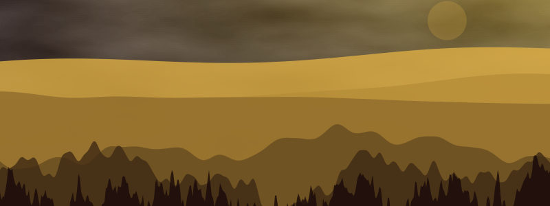

landscape(ColorSchemes.starrynight, "images/noise/landscapes-starrynight")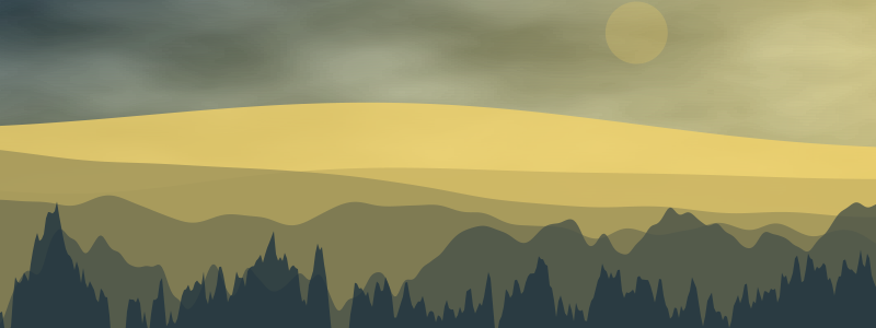

I generated a few hundred of these (there are over 300 colorschemes that can be selected at random) and, scrolling through them quickly, I found that sometimes the results were good, sometimes they weren't. Randomness—and noise—can be hard to predict.

[2018-10-16]

---

This page was generated using Literate.jl.